We performed epigenomic profiling carrying out ChIPseq for H3K27ac, H3K27me3 and H3K4me3 as well as ATACseq of OEP dissected tissue. Below we describe the enhancer discovery pipeline.
To view our cloned enhancer tracks, click here.
Our enhancer discovery pipeline integrates ChIP (H3K27ac and H3K27me3) and ATAC data into a single Nextflow sub-workflow. This sub-workflow is executed as part of the downstream analysis pipeline. If you would like to re-run the downstream analysis pipeline, follow the instructions here.
The sub-workflow uses Bedtools and Homer in order to identify putative enhancers:
Download putative enhancer co-ordinates
Download annotated putative enhancers
The sub-workflow also integrates custom R scripts for:
// Define DSL2
nextflow.enable.dsl=2
include {awk as awk_enhancer_filter; awk as awk_gtf_filter; awk as awk_trim_head; cut} from "$baseDir/../luslab-nf-modules/tools/luslab_linux_tools/main.nf"
include {bedtools_intersect} from "$baseDir/../luslab-nf-modules/tools/bedtools/main.nf"
include {bedtools_subtract} from "$baseDir/../luslab-nf-modules/tools/bedtools/main.nf"
include {homer_annotate_peaks; homer_find_motifs} from "$baseDir/../luslab-nf-modules/tools/homer/main.nf"
include {r_analysis as enhancer_profile; r_analysis as plot_motifs; r_analysis as functional_enrichment_analysis; r_analysis as peak_annotations_frequency} from "$baseDir/../modules/r_analysis/main.nf"
/*------------------------------------------------------------------------------------*/
/* Define sub workflow
--------------------------------------------------------------------------------------*/
workflow enhancer_analysis {
take:
chip_bigwig
atac_bigwig
chip_peaks
atac_peaks
genome
gtf
main:
// Keep only protein coding genes in gtf
awk_gtf_filter(params.modules['awk_gtf_filter'], gtf)
// // Intersect ATAC peaks with H3K27ac peaks
bedtools_intersect(params.modules['bedtools_intersect'], atac_peaks.filter{ it[0].sample_id == 'ATAC' }, chip_peaks.filter{ it[0].sample_id == 'H3K27Ac' }.map{ it[1] } )
// Remove any peaks which also have hits for H3K27me3
bedtools_subtract(params.modules['bedtools_subtract'], bedtools_intersect.out, chip_peaks.filter{ it[0].sample_id == 'H3K27me3' }.map{ it[1] } )
// Annotate remaining peaks
homer_annotate_peaks(params.modules['homer_annotate_peaks'], bedtools_subtract.out, genome, awk_gtf_filter.out.file_no_meta)
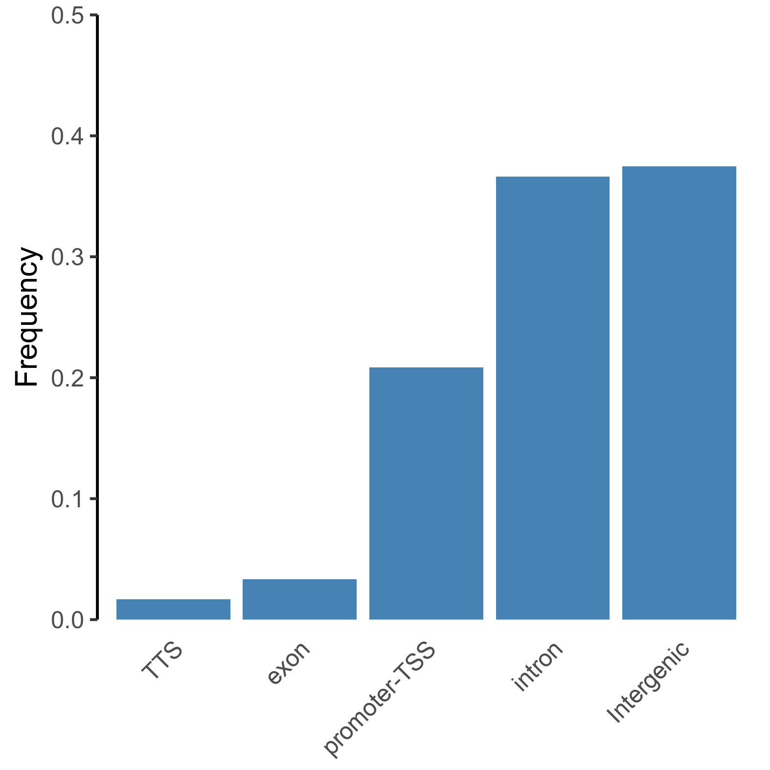
// Plot distribution of intersected peak annotations
peak_annotations_frequency(params.modules['peak_annotations_frequency'], homer_annotate_peaks.out.map{it[1]})
// Remove peaks in protein coding promoters and protein coding exons
awk_enhancer_filter(params.modules['awk_enhancer_filter'], homer_annotate_peaks.out)
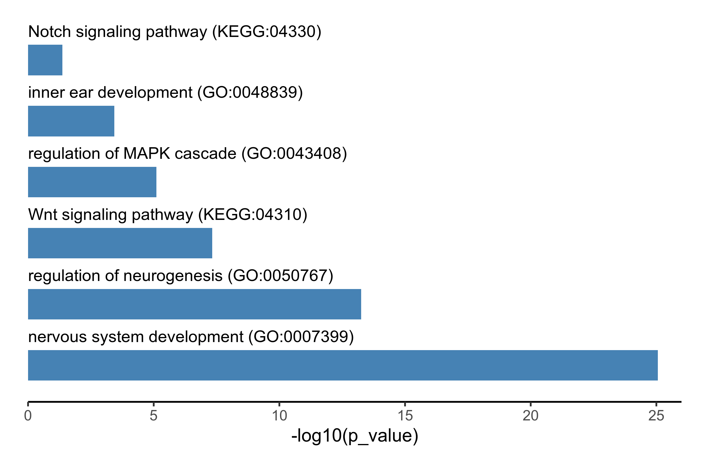
// Run functional enrichment analysis on annotated putative enhancers
functional_enrichment_analysis(params.modules['functional_enrichment_analysis'], awk_enhancer_filter.out.file_no_meta)
// Combine all peak data for enhancer profile input
enhancer_profile_input = chip_peaks.map{it[1]}.flatten().collect()
.combine(chip_bigwig.map{it[1]}.flatten().collect())
.combine(atac_peaks.map{it[1]}.flatten().collect())
.combine(atac_bigwig.map{it[1]}.flatten().collect())
.combine(awk_enhancer_filter.out.file_no_meta)
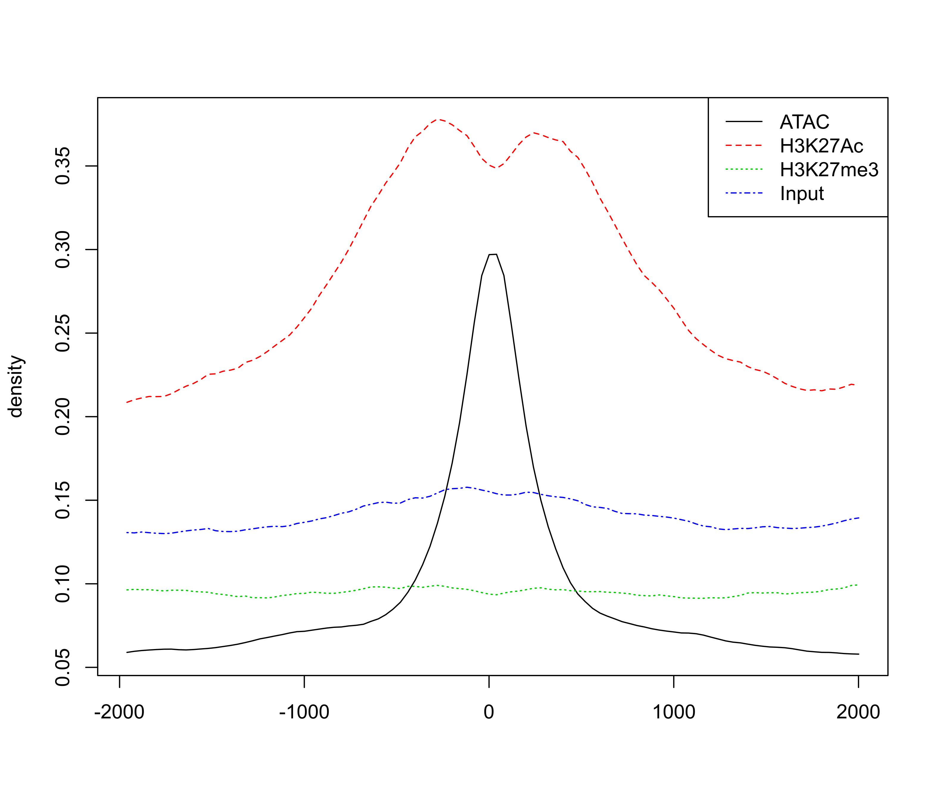
// Plot ChIP and ATAC profile across enhancers
enhancer_profile( params.modules['enhancer_profile'], enhancer_profile_input)
// Convert awk output to bed file
cut(params.modules['cut'], awk_enhancer_filter.out.file)
// Trim first line from bed file
awk_trim_head(params.modules['awk_trim_head'], cut.out.file)
// Run motif enrichment analysis on remaining peaks
homer_find_motifs(params.modules['homer_find_motifs'], awk_enhancer_filter.out.file, genome)
// Generate motif plot
plot_motifs( params.modules['plot_motifs'], homer_find_motifs.out.enrichedMotifs.map{it[1]} )
}
library(ggplot2)
library(extrafont)

output_path = './output/'
dir.create(output_path)

# import ATAC peaks intersected with +K27Ac -K27me3
peaks <- read.delim(list.files('./', pattern=".txt", full.names = TRUE), sep = "\t")

# extract and simplify annotations for categorisation
annotation_peaks <- as.factor(sub(' .*', "", peaks[,"Annotation"]))

# order frequency
freq_data <- as.data.frame(prop.table(table(annotation_peaks))[order(prop.table(table(annotation_peaks)))])
colnames(freq_data) = c('peaks', 'Frequency')


# plot frequency plot of peak annotations
png(paste0(output_path, "peak_annotation_frequency.png"), height = 10, width = 10, family = 'Arial', units = 'cm', res = 400)
ggplot(freq_data, aes(x = peaks, y = Frequency)) +
  geom_bar(stat='identity', fill='steelblue') +
  theme_classic() +
  theme(axis.title.x=element_blank(),
        axis.ticks.x=element_blank(),
        axis.line.x=element_blank(),
        axis.text.x = element_text(angle = 45, vjust = 0.95, hjust=1)) +
  scale_y_continuous(expand = c(0, 0), limits = c(0, 0.5))
graphics.off()
To view all of our functional enrichment analysis output in the browser, click here.
library(gprofiler2)
library(dplyr)
library(ggplot2)
library(extrafont)

output_path = './output/'
dir.create(output_path, recursive = T)

putative_enhancers <- read.delim(list.files(pattern = '*txt', full.names = TRUE))

# run functional enrichment analysis using GO:biological process and KEGG terms
fea_res <- gost(putative_enhancers$Entrez.ID, organism = 'ggallus', sources = c('GO:BP', 'KEGG'))

# generate URL for full results
# gost(putative_enhancers$Entrez.ID, organism = 'ggallus', sources = c('GO:BP', 'KEGG'), as_short_link = TRUE)

go_terms <- c("GO:0007399", "KEGG:04310", "GO:0048839", "GO:0050767", "GO:0043408", "KEGG:04330")

# select enriched terms of interest and generate bar plot
plot_data <- fea_res$result %>%
  filter(term_id %in% go_terms) %>%
  select(c(p_value, term_name, term_id)) %>%
  mutate(-log10(p_value)) %>%
  arrange(desc(`-log10(p_value)`)) %>%
  mutate(term_name = paste0(term_name, ' (', term_id, ")")) %>%
  mutate(term_name = factor(term_name, levels = term_name))

png(paste0(output_path, "functional_enrichment.png"), height = 10, width = 15, family = 'Arial', units = 'cm', res = 400)
ggplot(plot_data, aes(x = term_name, y = -log10(p_value), label = term_name)) +
  geom_bar(stat='identity', width=0.5, fill='steelblue') +
  coord_flip() +
  geom_text(aes(y = 0), hjust = 'left', vjust = -2, size = 3.5) +
  theme_classic() +
  theme(axis.title.y=element_blank(),
        axis.text.y=element_blank(),
        axis.ticks.y=element_blank(),
        axis.line.y=element_blank()) +
  scale_y_continuous(expand = c(0, 0), limits = c(0, 26)) +
  theme(plot.margin=unit(c(0.5,0.5,0.5,0.5),"cm"))
graphics.off()
library(ChIPpeakAnno)
library(rtracklayer)
library(extrafont)
output_path = "./output/"
dir.create(output_path, recursive = T)
# import putative enhancer peaks (ATAC peaks; + K27ac; - K27me3; - <2kb upstream TSS; - exons)
shared.peaks <- read.delim(list.files(pattern="*.txt", full.names = TRUE), sep = "\t")
peaks <- GRanges(seqnames=shared.peaks[,2],
ranges=IRanges(start=shared.peaks[,3],
end=shared.peaks[,4],
names=shared.peaks[,1]))
# find centre of ATAC peak and get coordinates for +/-2kb
peaks.recentered <- peaks.center <- peaks
start(peaks.center) <- start(peaks) + floor(width(peaks)/2)
width(peaks.center) <- 1
start(peaks.recentered) <- start(peaks.center) - 2000
end(peaks.recentered) <- end(peaks.center) + 2000
# import bigwig files and select regions corresponding to ATAC (putative enhancer) peaks
bigwig_files <- list.files('./', pattern = 'bigWig', full.names = T)
ATAC.bw <- import(bigwig_files[grepl("ATAC", bigwig_files)], format="BigWig", which=peaks.recentered, as="RleList")
H3K27Ac.bw <- import(bigwig_files[grepl("H3K27Ac", bigwig_files)], format="BigWig", which=peaks.recentered, as="RleList")
H3K27me3.bw <- import(bigwig_files[grepl("H3K27me3", bigwig_files)], format="BigWig", which=peaks.recentered, as="RleList")
input.bw <- import(bigwig_files[grepl("input", bigwig_files)], format="BigWig", which=peaks.recentered, as="RleList")
# make list of bigwig files
bw <- list(ATAC = ATAC.bw, H3K27Ac = H3K27Ac.bw, H3K27me3 = H3K27me3.bw, Input = input.bw)
# extract signal for +/-2kb around enhancer peak for visualisation
sig <- featureAlignedSignal(bw, peaks.recentered,
upstream=2000, downstream=2000)
# plot profile around ATAC peaks
png(paste0(output_path, "metaprofile.png"), width=20, height=17, family = 'Arial', units = 'cm', res = 400)
featureAlignedDistribution(sig, peaks.recentered, upstream=2000, downstream=2000, type="l")
graphics.off()
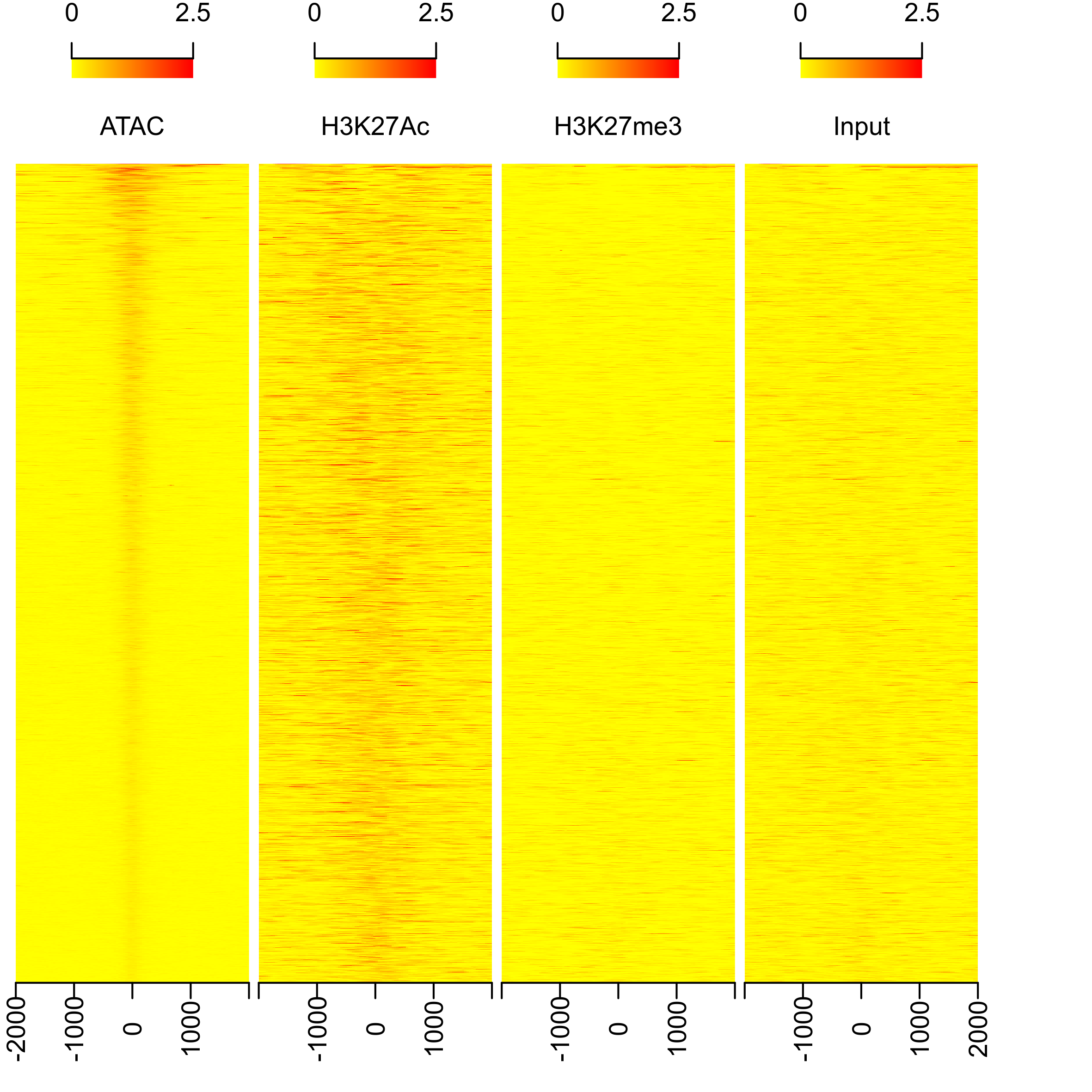
# plot heatmap
png(paste0(output_path, "heatmap.png"), width=15, height=15, family = 'Arial', units = 'cm', res = 400)
featureAlignedHeatmap(sig, peaks.recentered, upstream=2000, downstream=2000, upper.extreme=2.5)
graphics.off()
library(ggseqlogo)
library(gridExtra)
library(cowplot)
library(ggplot2)
library(extrafont)

output_path = "./output/"
dir.create(output_path, recursive = T)


######## read in data
# read in logo data
motif_logos = list()
for(i in 1:20){
  motif_logos[[paste(i)]] <- t(read.delim(paste0('./ATAC_motif_enrichment/knownResults/known', i, '.motif'))[1:4])
  rownames(motif_logos[[paste(i)]]) = c('A', 'C', 'G', 'T')
}

# read in motif info
motif_meta = read.delim(paste0('./ATAC_motif_enrichment/knownResults.txt'))[1:20,c(1,3)]

# strip name
motif_meta[,1] <- sub("\\(.*", "", motif_meta[,1])


####### prepare grobs
# gene names
gene = list(as_grob(~plot(c(0, 1), c(0, 1), ann = F, bty = 'n', type = 'n', xaxt = 'n', yaxt = 'n') +
  text(x = 0.5, y = 0.5, "Gene", cex = 15, col = "black", font=2)))

motif_names <- lapply(motif_meta[,1], function(x) {as_grob(~plot(c(0, 1), c(0, 1), ann = F, bty = 'n', type = 'n', xaxt = 'n', yaxt = 'n') +
                                 text(x = 0.5, y = 0.5, x, cex = 10, col = "black"))})


# motifs
motif = list(as_grob(~plot(c(0, 1), c(0, 1), ann = F, bty = 'n', type = 'n', xaxt = 'n', yaxt = 'n') +
                 text(x = 0.5, y = 0.5, "Motif", cex = 15, col = "black", font=2)))

motif_logos = lapply(motif_logos, function(x) {ggseqlogo(x, method = 'prob') + theme_void() + theme(plot.margin = unit(c(2,0,2,0), "cm"))})


# pvalues
pval = list(as_grob(~plot(c(0, 1), c(0, 1), ann = F, bty = 'n', type = 'n', xaxt = 'n', yaxt = 'n') +
                      text(x = 0.5, y = 0.5, "p-value", cex = 15, col = "black", font=2)))

motif_pval <- lapply(motif_meta[,2], function(x) {as_grob(~plot(c(0, 1), c(0, 1), ann = F, bty = 'n', type = 'n', xaxt = 'n', yaxt = 'n') +
                                                             text(x = 0.5, y = 0.5, x, cex = 10, col = "black"))})

######## plot grobs
png(paste0(output_path, 'top20_motifs.png'), width = 180, height = 300, family = 'Arial', units = 'cm', res = 200)
grid.arrange(grobs=c(gene, motif_names, motif, motif_logos, pval, motif_pval), ncol=3, widths = c(1, 3, 1), as.table=FALSE)
graphics.off()

########  plot selected motifs
motifs_of_interest <- c('Sox3', 'Sox2', 'Sox10', 'TEAD3', 'Six2', 'Six1', 'Sox9', 'AP-2alpha')
motifs_of_interest <- which(motif_meta$Motif.Name %in% motifs_of_interest)

png(paste0(output_path, 'selected_motifs.png'), width = 150, height = 150, family = 'Arial', units = 'cm', res = 400)
grid.arrange(grobs=c(gene, motif_names[motifs_of_interest], motif, motif_logos[motifs_of_interest], pval, motif_pval[motifs_of_interest]), ncol=3, widths = c(1, 4, 1), as.table=FALSE)
graphics.off()

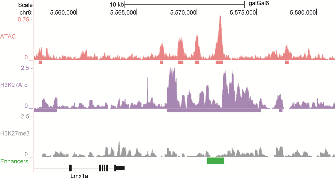
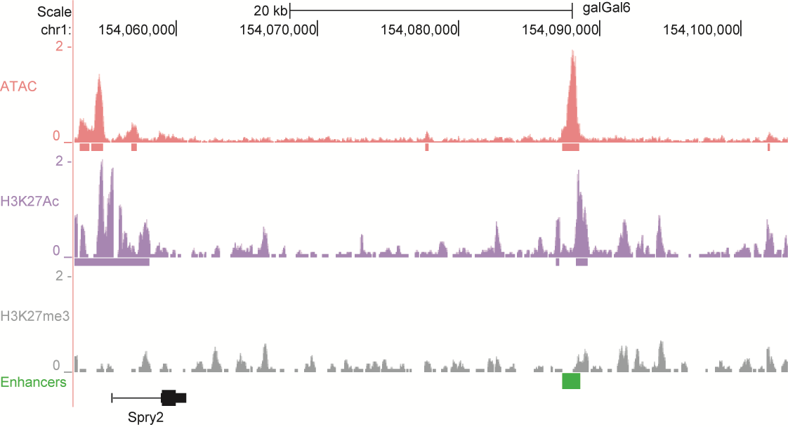
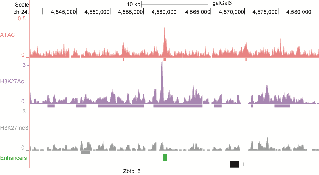
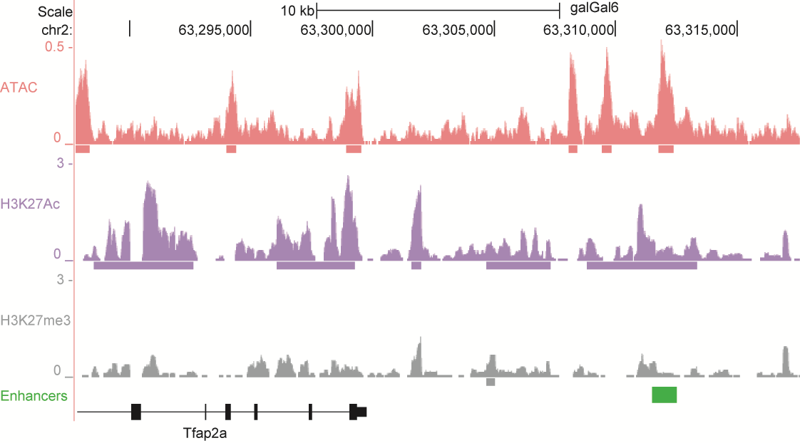
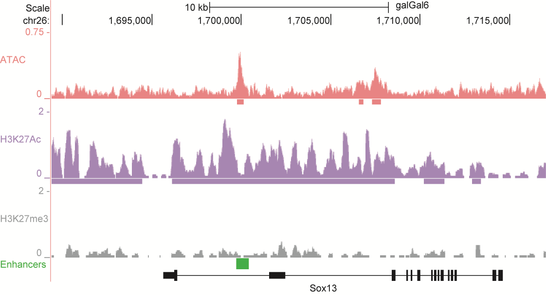
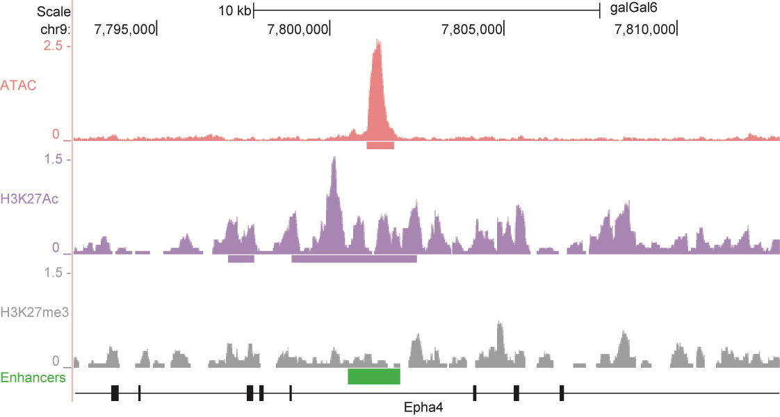
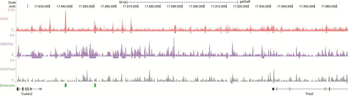
After identifying putative enhancers, we visualised them in the UCSC genome browser before cloning and validating selected enhancers. Below are the genome tracks of validated cloned enhancers and the correponding ChIP/ATAC peaks.
Download all cloned enhancer tracks.
×