To assess the transcriptomic changes that accompany the development of OEPs, we performed single cell RNAseq. To do so, we took advantage of a Pax2E1-EGFP enhancer to genetically label OEP, Otic and Epibranchial cells. Embryos were electroporated at head-fold stages and EGFP+ cells were collected at ss8-9, ss11-12 and ss14-16 by FACS and processed for SmartSeq2 single cell RNAseq.
The data was analysed primarily using the Antler R package, which has been developed specifically for analysing single cell RNAseq experiments. This package aims to perform unbiased data driven analysis.
The version of Antler used in this analysis corresponds to the version published in Delile et al. 2019.
Pseudotemporal analysis is carried out using Monocle2 (Qiu et al. 2017).
RNA velocity is carried out using Velocyto (La Manno et al. 2018).
Automatic switch for running pipeline through Nextflow or interactively in Rstudio.
library(getopt)
spec = matrix(c(
  'runtype', 'l', 2, "character",
  'cores'   , 'c', 2, "integer",
  'custom_functions', 'm', 2, "character"
), byrow=TRUE, ncol=4)
opt = getopt(spec)

# Set run location
if(length(commandArgs(trailingOnly = TRUE)) == 0){
  cat('No command line arguments provided, user defaults paths are set for running interactively in Rstudio on docker\n')
  opt$runtype = "user"
} else {
  if(is.null(opt$runtype)){
    stop("--runtype must be either 'user' or 'nextflow'")
  }
  if(tolower(opt$runtype) != "user" & tolower(opt$runtype) != "nextflow"){
    stop("--runtype must be either 'user' or 'nextflow'")
  }
  if(tolower(opt$runtype) == "nextflow"){
    if(is.null(opt$custom_functions) | opt$custom_functions == "null"){
      stop("--custom_functions path must be specified in process params config")
    }
  }
}
Set paths and pipeline parameters. Load data, packages and custom functions.
{
  if (opt$runtype == "user"){

    # load custom functions
    sapply(list.files('./NF-downstream_analysis/bin/custom_functions/', full.names = T), source)

    # set input data paths
    merged_counts_path = './alignment_output/NF-smartseq2_alignment/merged_counts/output/'
    gfp_counts = './alignment_output/NF-smartseq2_alignment/merged_counts/output/'
    velocyto_input = './alignment_output/NF-smartseq2_alignment/velocyto/'
    genome_annotations_path = './alignment_output/NF-downstream_analysis/extract_gtf_annotations/'

    # set output data paths
    output_path = "./output/NF-downstream_analysis/smartseq_analysis/output/"
    plot_path = "./output/NF-downstream_analysis/smartseq_analysis/output/plots/"

    # set cores
    ncores = 8

  } else if (opt$runtype == "nextflow"){
    cat('pipeline running through nextflow\n')

    # load custom functions
    sapply(list.files(opt$custom_functions, full.names = T), source)
    output_path = "./output/"
    plot_path = "./output/plots/"
    merged_counts_path = './'
    genome_annotations_path = './'
    gfp_counts = './'
    velocyto_input = './'

    # set cores
    ncores = opt$cores
  }

  dir.create(output_path, recursive = T)
  dir.create(plot_path, recursive = T)

  # load required packages
  library(Antler)
  library(velocyto.R)
  library(stringr)
  library(monocle)
  library(plyr)
  library(dplyr)
  library(ggsignif)
  library(cowplot)
  library(rstatix)
  library(extrafont)
}

# set pipeline params
seed=1
perp=5
eta=200

#' Stage colors
stage_cols = setNames(c("#BBBDC1", "#6B98E9", "#05080D"), c('8', '11', '15'))
Load data and initialise Antler object.
# Load and hygienize dataset
m = Antler$new(plot_folder=plot_path, num_cores=ncores)

# load in phenoData and assayData from ../dataset -> assayData is count matrix; phenoData is metaData (i.e. replicated, conditions, samples etc)
m$loadDataset(folderpath=merged_counts_path)

pData(m$expressionSet)$cells_colors = stage_cols[as.character(pData(m$expressionSet)$timepoint)]
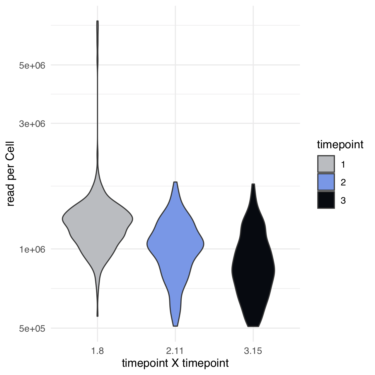
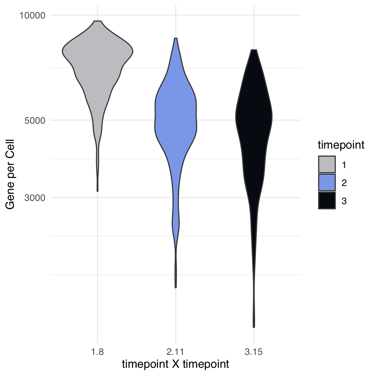
Plot pre-QC metrics.
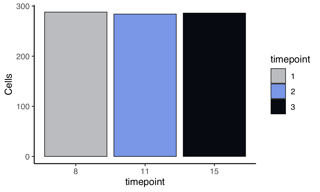
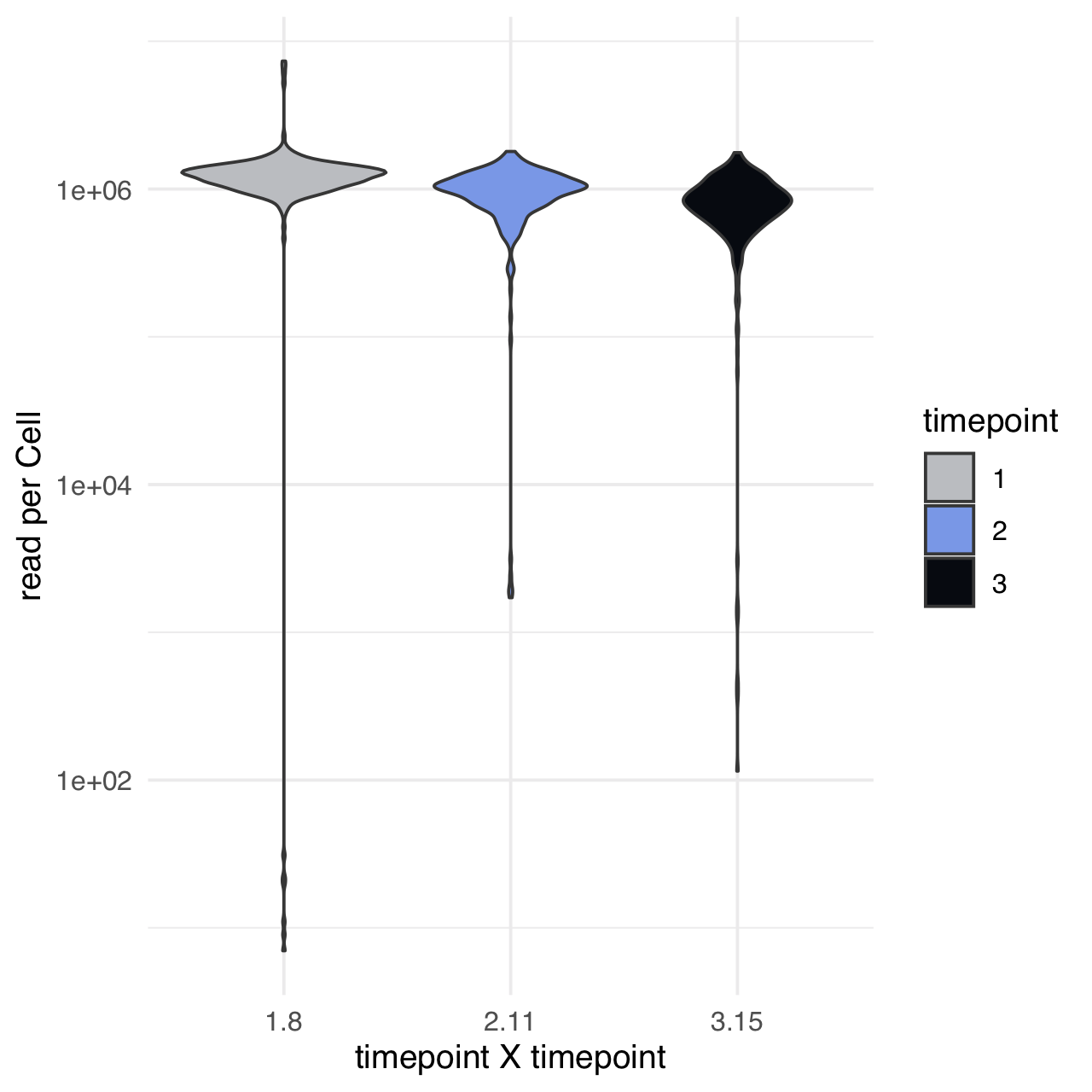
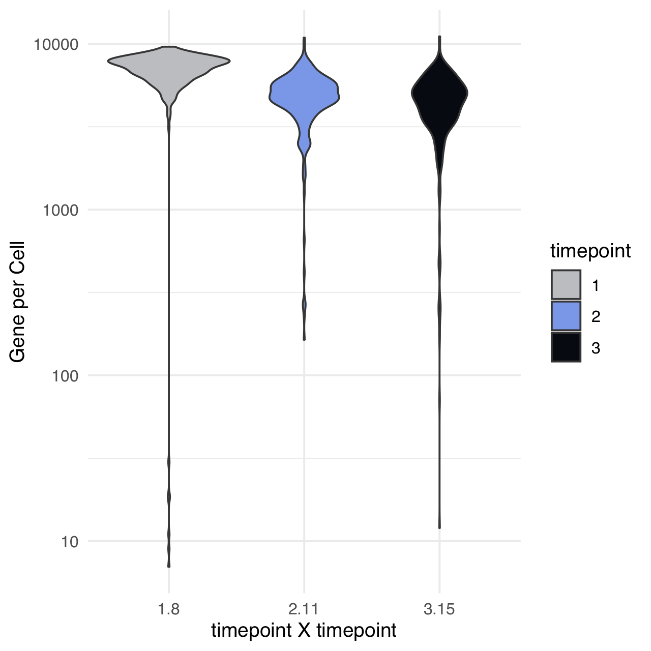
m$plotReadcountStats(data_status="Raw", by="timepoint", category="timepoint", basename="preQC", reads_name="read", cat_colors=unname(stage_cols))
Some key genes are not annotated in the GTF - we manually add these gene names to the annotations file.
# read in annotations file
gtf_annotations = read.csv(list.files(genome_annotations_path, pattern = '*gene_annotations.csv', full.names = T), stringsAsFactors = F)

# add missing annotations to annotations file
extra_annotations = c('FOXI3' = 'ENSGALG00000037457', 'ATN1' = 'ENSGALG00000014554', 'TBX10' = 'ENSGALG00000038767',
                      'COL11A1' = 'ENSGALG00000005180', 'GRHL2' = 'ENSGALG00000037687')

# add extra annotations to annotations csv file
gtf_annotations[,2] <- apply(gtf_annotations, 1, function(x) ifelse(x[1] %in% extra_annotations, names(extra_annotations)[extra_annotations %in% x], x[2]))

# label extra MT genes
MT_genes = c('ND3', 'CYTB', 'COII', 'ATP8', 'ND4', 'ND4L')
gtf_annotations[gtf_annotations[,2] %in% MT_genes,2] <- paste0('MT-', gtf_annotations[gtf_annotations[,2] %in% MT_genes,2])

write.csv(gtf_annotations, paste0(output_path, 'new_annotations.csv'), row.names = F)

# set gene annotations
m$setCurrentGeneNames(geneID_mapping_file=paste0(output_path, 'new_annotations.csv'))
Add list of key genes to Antler object.
#' Store known genes
apriori_genes = c(
  'DACH1', 'DLX3', 'DLX5', 'DLX6', 'EYA1', 'EYA2', 'FOXG1', 'FOXI3', 'GATA3', 'GBX2', 'HESX1', 'IRX1', 'IRX2', 'IRX3', 'LMX1A', 'LMX1B', 'PAX2', 'SALL4', 'SIX4', 'SOHO-1', 'SOX10', 'SOX2', 'SOX8', 'SOX9', 'SIX1', 'TBX2', # Known_otic_genes
  'ATN1', 'BACH2', 'CNOT4', 'CXCL14', 'DACH2', 'ETS1', 'FEZ1', 'FOXP3', 'HIPK1', 'HOMER2', 'IRX4', 'IRX5', 'KLF7', 'KREMEN1', 'LDB1', 'MSI1', 'PDLIM4', 'PLAG1', 'PNOC', 'PKNOX2', 'RERE', 'SMOC1', 'SOX13', 'TCF7L2', 'TEAD3', 'ZBTB16', 'ZFHX3', 'ZNF384', 'ZNF385C', # New_otic_TFs
  'PRDM1', 'FOXI1', 'NKX2-6', 'NR2F2', 'PDLIM1', 'PHOX2B', 'SALL1', 'TBX10', 'TFAP2E', 'TLX1', 'VGLL2', # Epibranchial_genes
  'ZNF423', 'CXCR4', 'MAFB', 'MYC', 'ZEB2', # Neural_Genes
  'CD151', 'ETS2', 'FGFR4', 'OTX2', 'Pax3', 'PAX6', 'PAX7', 'SIX3', # Non_otic_placode_genes
  'FOXD3', 'ID2', 'ID4', 'MSX1', 'TFAP2A', 'TFAP2B', 'TFAP2C', # Neural_Crest_Genes
  'GATA2', # Epidermis_genes
  'COL11A1', 'DTX4', 'GRHL2', 'NELL1', 'OTOL1', # Disease_associated_genes
  'ARID3A', 'BMP4', 'CREBBP', 'ETV4', 'ETV5', 'EYA4', 'FOXP4', 'FSTL4', 'HOXA2', 'JAG1', 'LFNG', 'LZTS1', 'MAFA', 'MEIS1', 'MYB', 'MYCN', 'NFKB1', 'NOTCH1', 'SPRY1', 'SPRY2', 'SSTR5', # chen et al. 2017
  'TWIST1', 'ASL1', 'MAF' # other_genes
)

m$favorite_genes <- unique(sort(apriori_genes))
Remove gene and cell outliers.
#' Remove outliers genes and cells
m$removeOutliers( lowread_thres = 5e5,   # select cells with more than 500000 reads
                  genesmin = 1000,       # select cells expressing more than 1k genes
                  cellmin = 3,           # select genes expressed in more than 3 cells)
                  data_status='Raw')
Remove control cells.
annotations = list(
  "blank"=c('241112', '250184', '265102', '272111', '248185', '274173'),
  "bulk"=c('225110', '251172', '273103', '280110', '235161', '246161'),
  "human"=c('233111', '249196', '257101', '264112', '233185', '247173')
)

m$excludeCellsFromIds(which(m$getCellsNames() %in% unlist(annotations)))
Remove cells with more than 6% of mitochondrial read counts.
m$removeGenesFromRatio(
  candidate_genes=grep('^MT-', m$getGeneNames(), value=T),
  threshold = 0.06
)
QC plots.
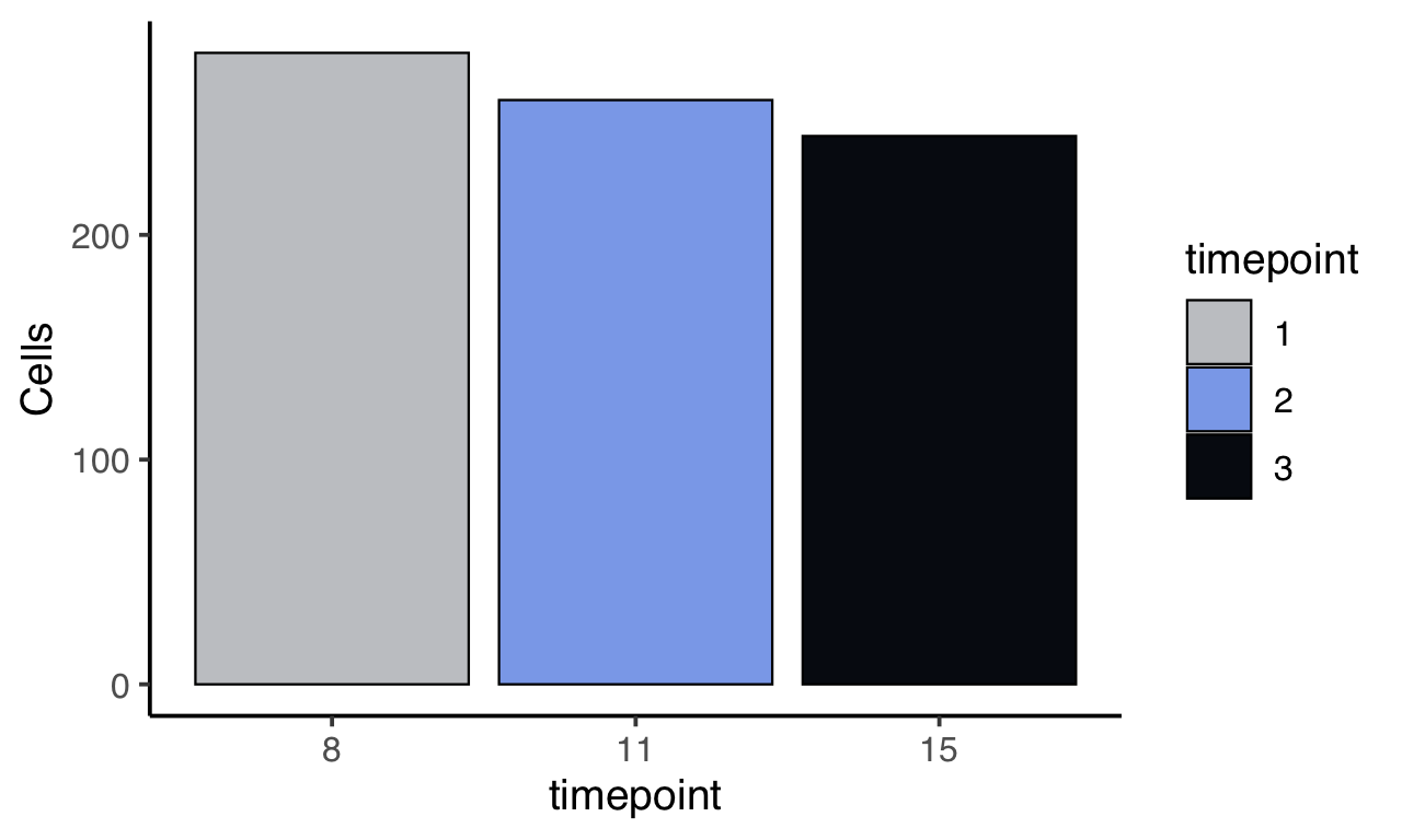
m$plotReadcountStats(data_status="Raw", by="timepoint", category="timepoint", basename="postQC", reads_name="read", cat_colors=unname(stage_cols))
Normalize readcounts to CPM and remove genes with <10 CPM.
m$normalize(method="Count-Per-Million")
m$excludeUnexpressedGenes(min.cells=3, data_status='Normalized')
m$removeLowlyExpressedGenes(expression_threshold=1, selection_theshold=10, data_status='Normalized')
Generate gene-gene correlation matrix.
# change plot folder
curr_plot_folder = paste0(plot_path, "all_cells/")
dir.create(curr_plot_folder)

# "fastCor" uses the tcrossprod function which by default relies on BLAS to speed up computation. This produces inconsistent result in precision depending on the version of BLAS being used.
# see "matprod" in https://stat.ethz.ch/R-manual/R-devel/library/base/html/options.html
corr.mat = fastCor(t(m$getReadcounts(data_status='Normalized')), method="spearman")
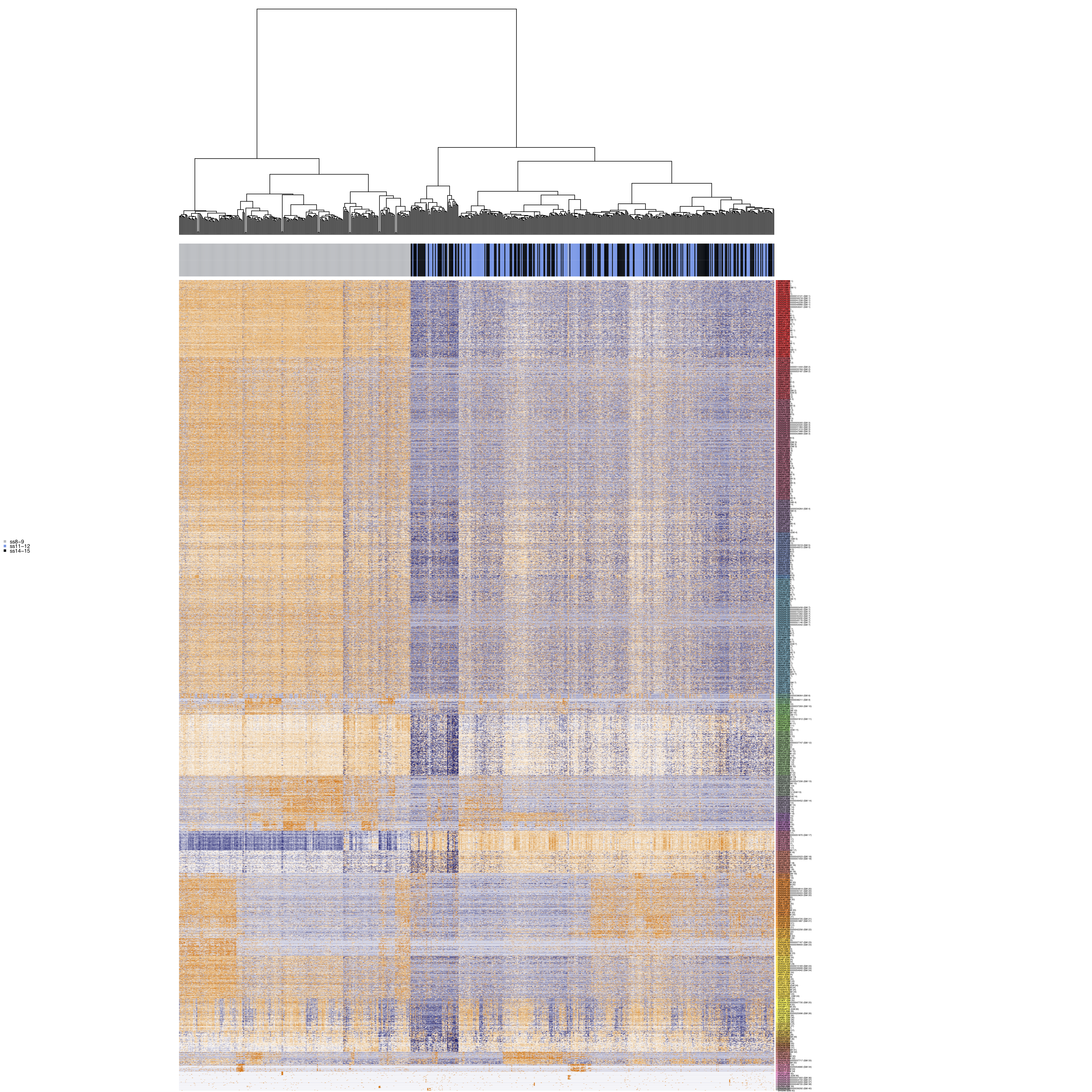
Identification of modules of co-correlated genes
Using the Antler package, we are able to cluster genes and identify sets of co-correlated genes termed gene modules. This works by heirarchically clustering a gene-gene correlation matrix, followed by iterative filtering of poor quality clusters.
For further information on Antler gene module identification, click here.
#' ## Gene modules identification
m$identifyGeneModules(
  method="TopCorr_DR",
  corr=corr.mat,
  corr_t = 0.3, # gene correlation threshold
  topcorr_mod_min_cell=0, # default
  topcorr_mod_consistency_thres=0.4, # default
  topcorr_mod_skewness_thres=-Inf, # default
  topcorr_min_cell_level=5,
  topcorr_num_max_final_gms=40, # heuristically set to give sufficient cluster diversity and of reasonable size in order to select modules from gene candidate list
  data_status='Normalized'
)
# corr_t = gene correlation threshold
# topcorr_mod_min_cell = minimum number of cells expressing gene module
# topcorr_mod_consistency_thres = proportion of cells expressing gene module (binarised z-scored log-transformed normalised expression levels)
# topcorr_mod_skewness_thres = test whether genes are expressed only in subset of cells
# topcorr_min_cell_level = minimum expression level in cells which express gene module
# topcorr_num_max_final_gms = maximum number of final gene modules

names(m$topCorr_DR$genemodules) <- paste0("GM ", seq(length(m$topCorr_DR$genemodules)))
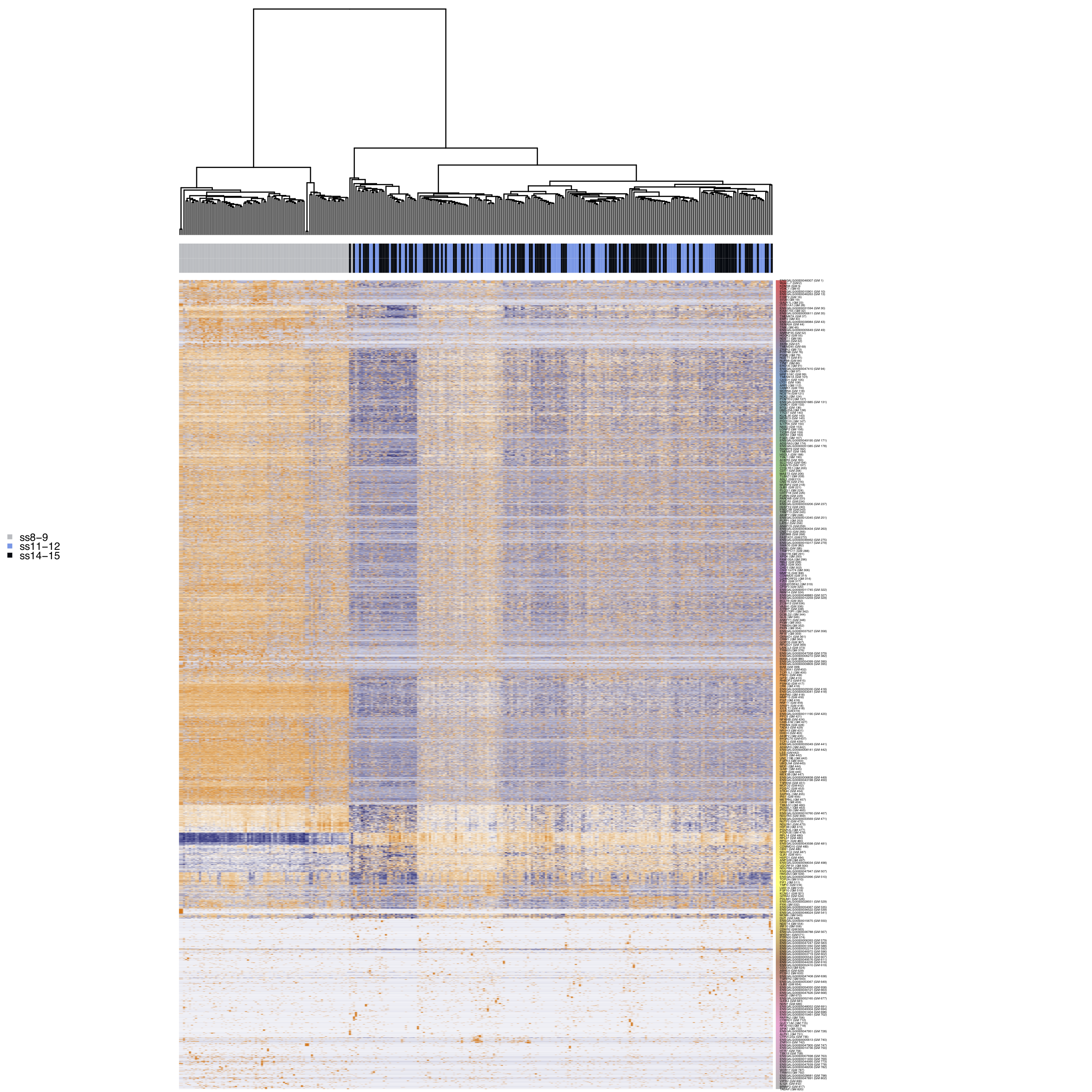
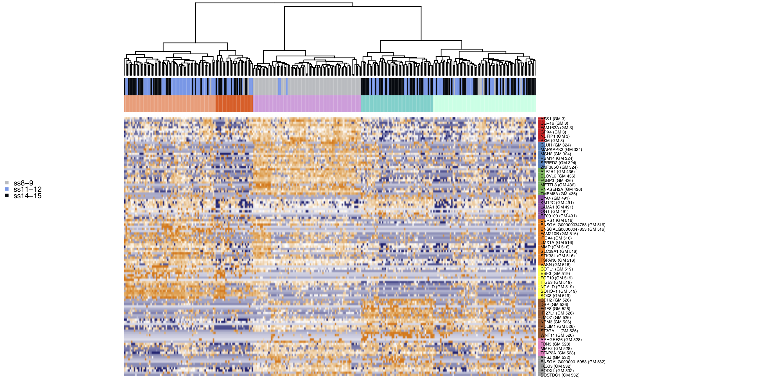
Plot gene modules.
# identify cell clusters based on remaining genes
m$identifyCellClusters(method='hclust', used_genes="topCorr_DR.genemodules", data_status='Normalized')

m$plotGeneModules(
  basename='AllCells',
  curr_plot_folder = curr_plot_folder,
  displayed.gms = 'topCorr_DR.genemodules',
  displayed.geneset=NA,
  use.dendrogram='hclust',
  display.clusters=NULL,
  file_settings=list(list(type='pdf', width=20, height=20)),
  data_status='Normalized',
  gene_transformations='logscaled',
  pretty.params=list("size_factor"=3, "ngenes_per_lines" = 0, "side.height.fraction"=.15),
  display.legend = FALSE,
  extra_legend=list("text"=c('ss8-9', 'ss11-12', 'ss14-15'), "colors"=unname(stage_cols))
)

m$writeGeneModules(basename='AllCells_allGms', gms='topCorr_DR.genemodules', folder_path = curr_plot_folder)
Filter out cells with low summary counts.
m2 = m$copy()
m2$excludeCellsFromIds(m$getReadcounts('Normalized')[unlist(m$topCorr_DR$genemodules),] %>% colSums %>% {as.numeric(scale(log(.), center=TRUE, scale=T))} %>% {which(. < -1.5)})
m2$excludeUnexpressedGenes(min.cells=1, data_status="Normalized", verbose=TRUE)
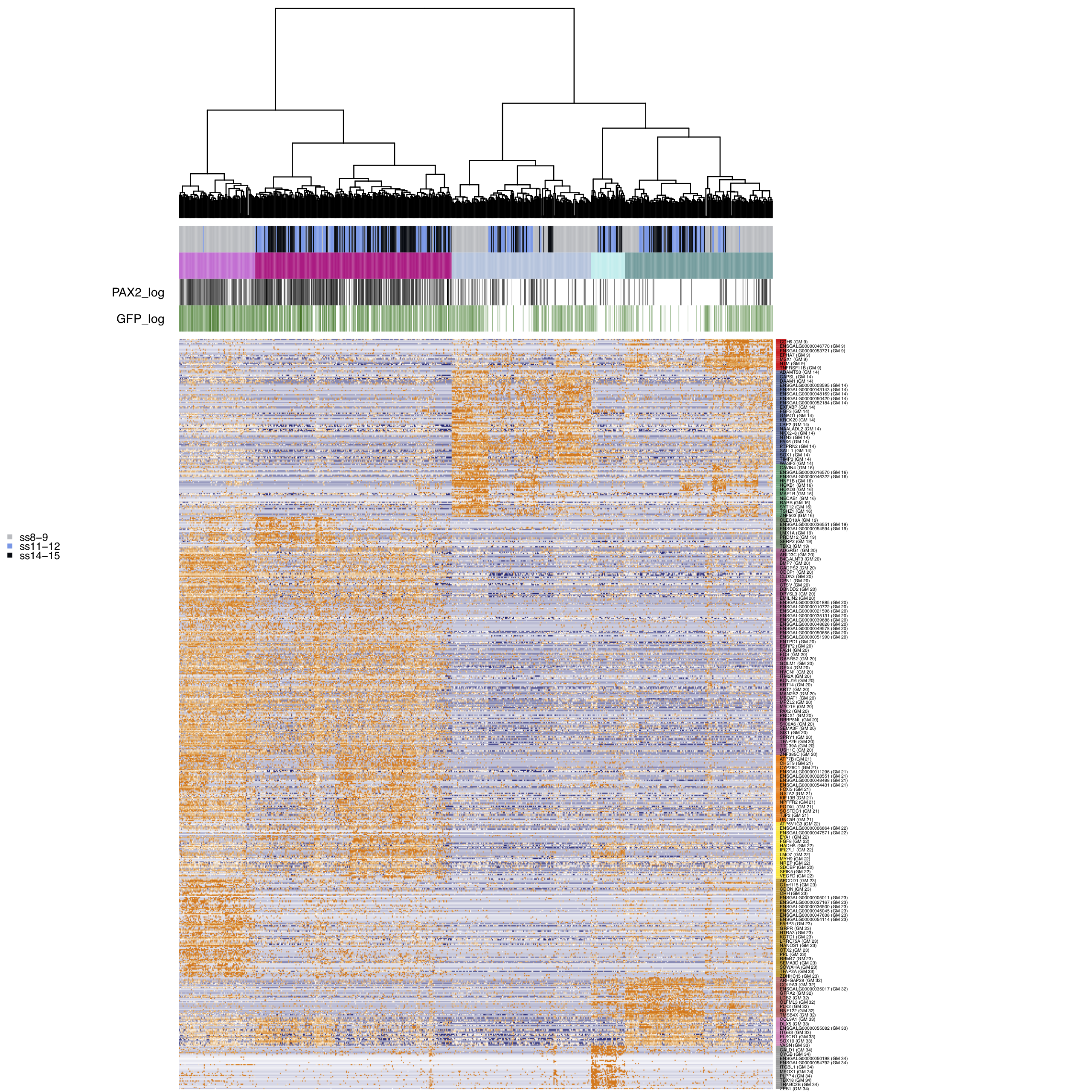
We select gene modules based on the presence of genes known to be involved in the development of ectodermal lineages. After subsetting the gene modules we re-cluster the cells.
bait_genes = c("HOXA2", "PAX6", "SOX2", "MSX1", "Pax3", "SALL1", "ETS1", "TWIST1", "HOMER2", "LMX1A", "VGLL2", "EYA2", "PRDM1", "FOXI3", "NELL1", "DLX5", "SOX8", "SOX10", "SOHO-1", "IRX4", "DLX6")

m2$dR$genemodules = Filter(function(x){any(bait_genes %in% x)}, m2$topCorr_DR$genemodules)

# cluster into 5 clusters
m2$identifyCellClusters(method='hclust', clust_name="Mansel", used_genes="dR.genemodules", data_status='Normalized', numclusters=5)

# set cluster colours
clust.colors <- c('#da70d6', '#c71585', '#b0c4de', '#afeeee', '#5f9ea0')

# read in GFP counts
gfp_counts = read.table(file=paste0(gfp_counts, 'gfpData.csv'), header=TRUE, check.names=FALSE)
Plot final clustering of all cells.
m2$plotGeneModules(
  basename='AllCellsManualGMselection',
  curr_plot_folder = curr_plot_folder,
  displayed.gms = 'dR.genemodules',
  displayed.geneset=NA,
  use.dendrogram='Mansel',
  file_settings=list(list(type='pdf', width=10, height=10)),
  data_status='Normalized',
  gene_transformations=c('log', 'logscaled'),
  extra_colors=cbind(
    m2$cellClusters$Mansel$cell_ids %>% clust.colors[.],
"PAX2_log"=m2$getReadcounts(data_status='Normalized')['PAX2',] %>%
      {log10(1+.)} %>%
      {as.integer(1+100*./max(.))} %>%
      colorRampPalette(c("white", "black"))(n=100)[.],
    "GFP_log"= as.numeric(gfp_counts[m2$getCellsNames()]) %>%
{log10(1+.)} %>%
{as.integer(1+100*./max(.))} %>%
colorRampPalette(c("white", "darkgreen"))(n=100)[.]
),
pretty.params=list("size_factor"=2, "side.height.fraction"=0.5),
display.legend = FALSE,
extra_legend=list("text"=c('ss8-9', 'ss11-12', 'ss14-15'), "colors"=unname(stage_cols))
)

m2$writeGeneModules(basename='AllCells_baitGMs', gms='dR.genemodules', folder_path = curr_plot_folder)
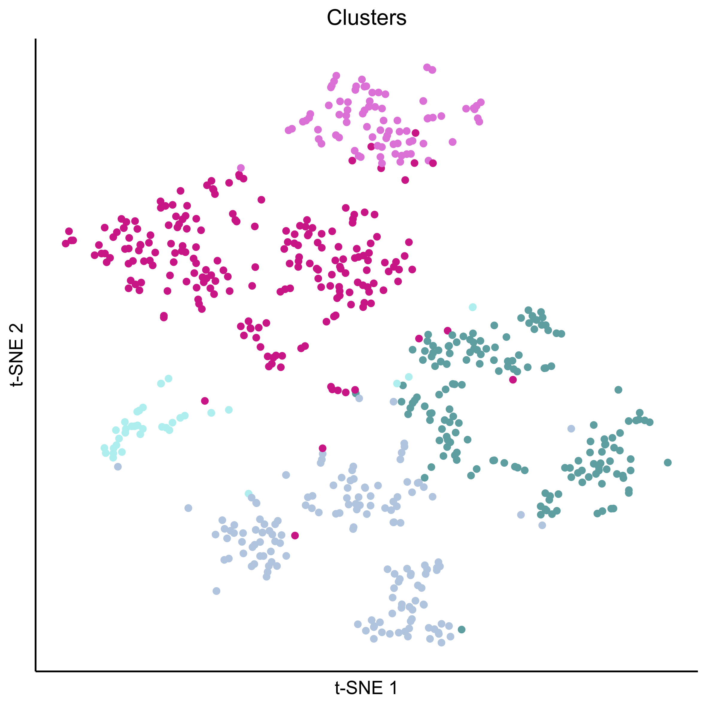
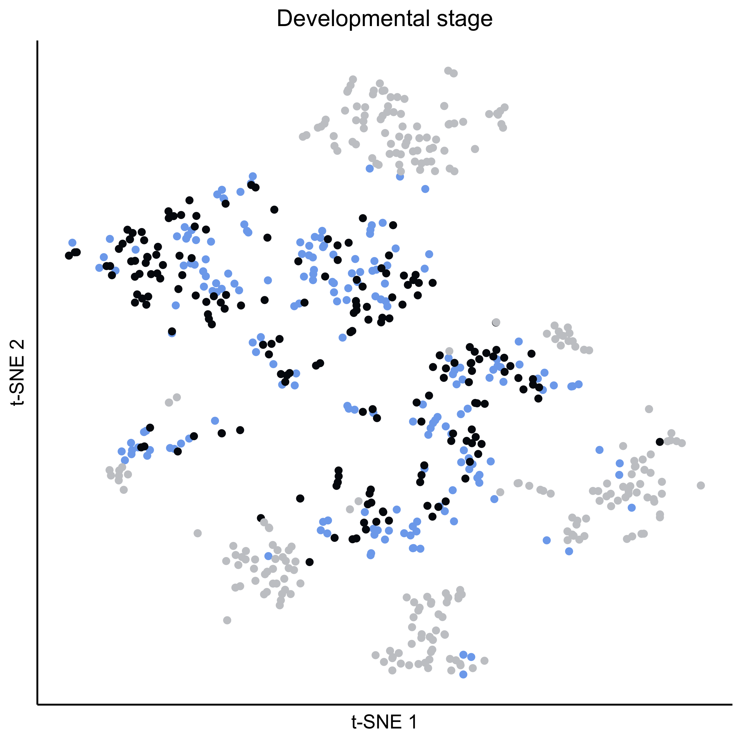
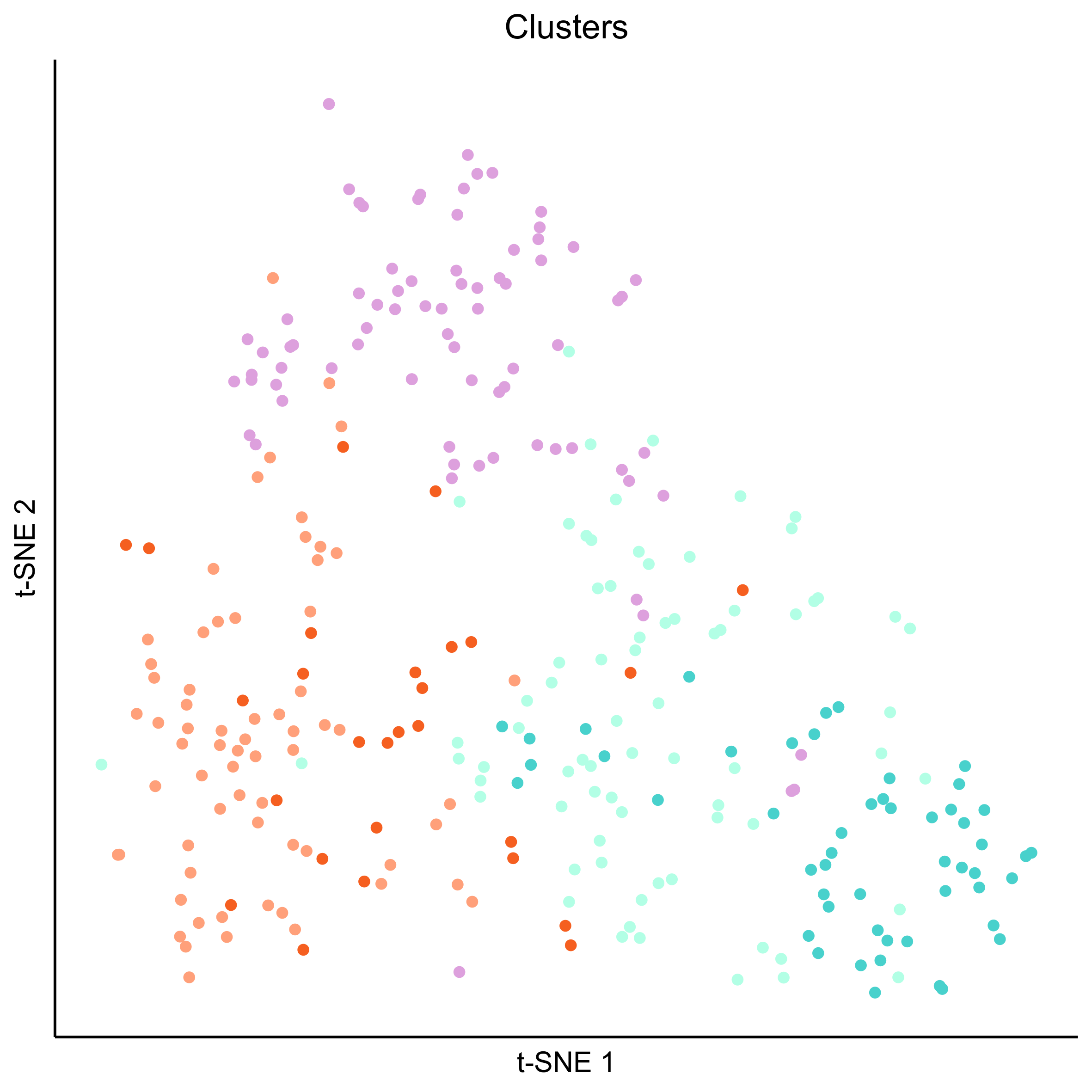
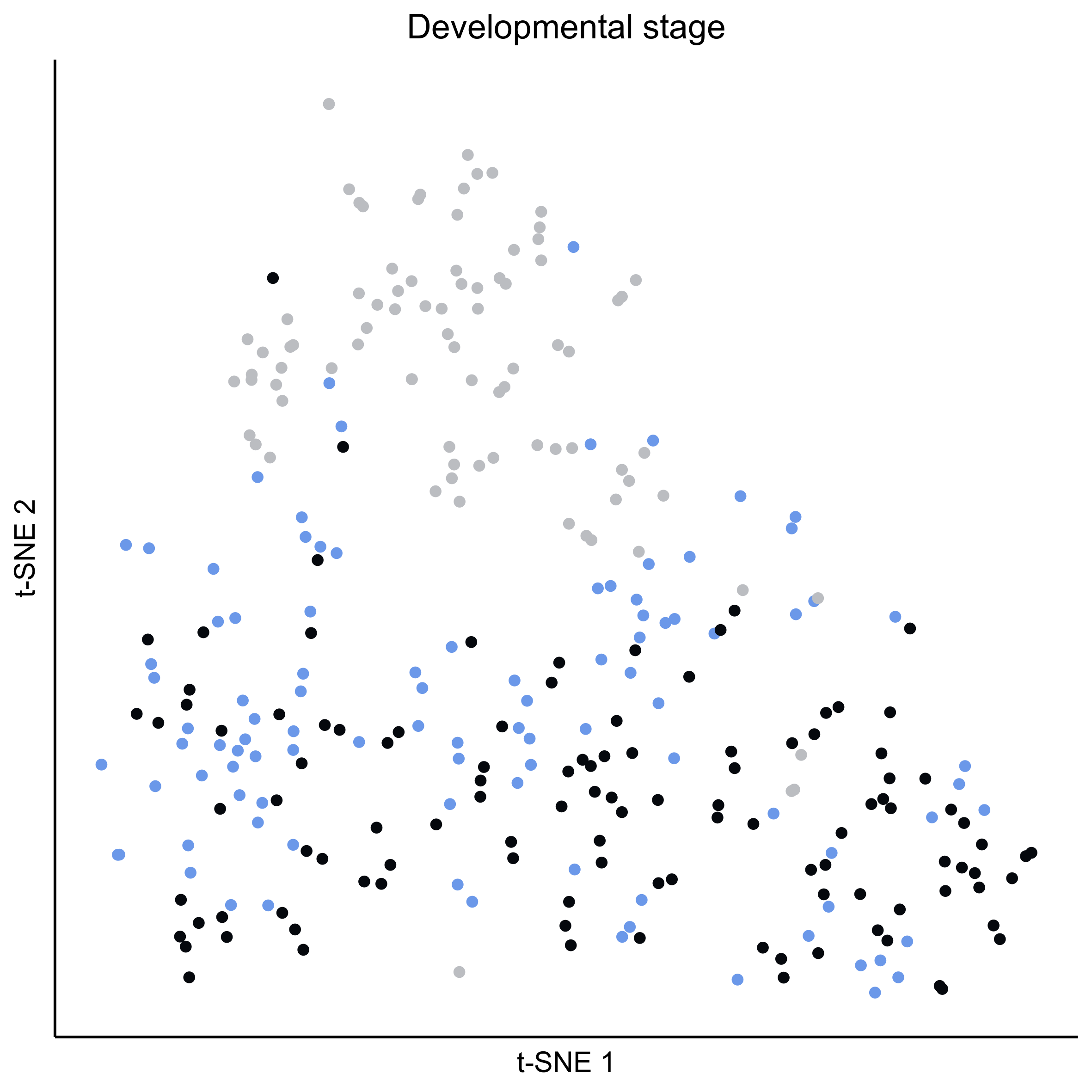
Plot tSNEs of cell clusters and developmental stage.
curr_plot_folder = paste0(plot_path, "all_cells/tsne/")
dir.create(curr_plot_folder)


png(paste0(curr_plot_folder, 'allcells_clusters_TSNE.png'), height = 15, width = 15, family = 'Arial', units = 'cm', res = 400)
tsne_plot(m2, m2$dR$genemodules, seed=seed, colour_by=m2$cellClusters$Mansel$cell_ids, colours=clust.colors, perplexity=perp, eta=eta) +
  ggtitle('Clusters') +
  theme(plot.title = element_text(hjust = 0.5))
graphics.off()


png(paste0(curr_plot_folder, 'allcells_stage_TSNE.png'), height = 15, width = 15, family = 'Arial', units = 'cm', res = 400)
tsne_plot(m2, m2$dR$genemodules, seed=seed, colour_by = pData(m2$expressionSet)$timepoint, colours = stage_cols, perplexity=perp, eta=eta) +
  ggtitle('Developmental stage') +
  theme(plot.title = element_text(hjust = 0.5))
graphics.off()
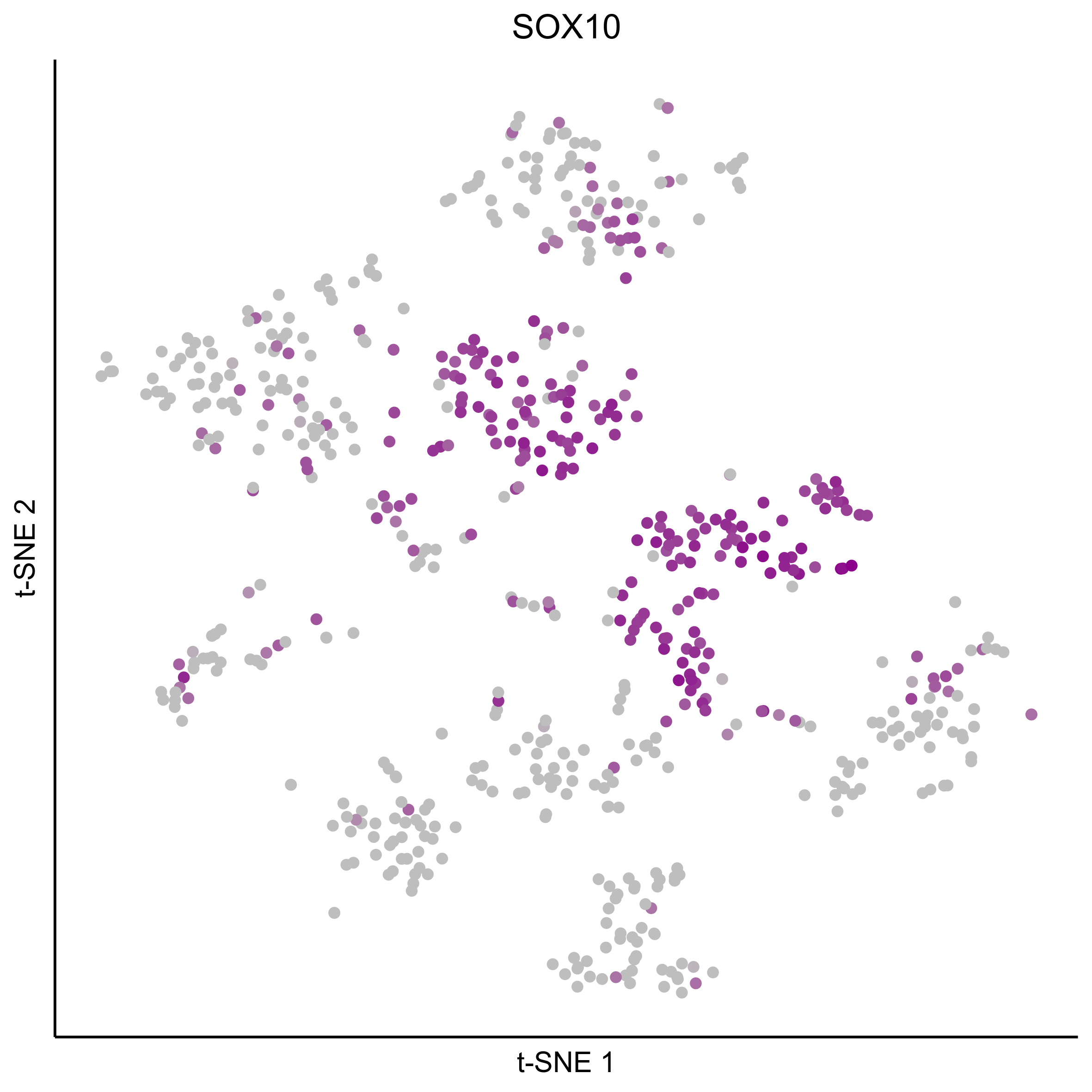
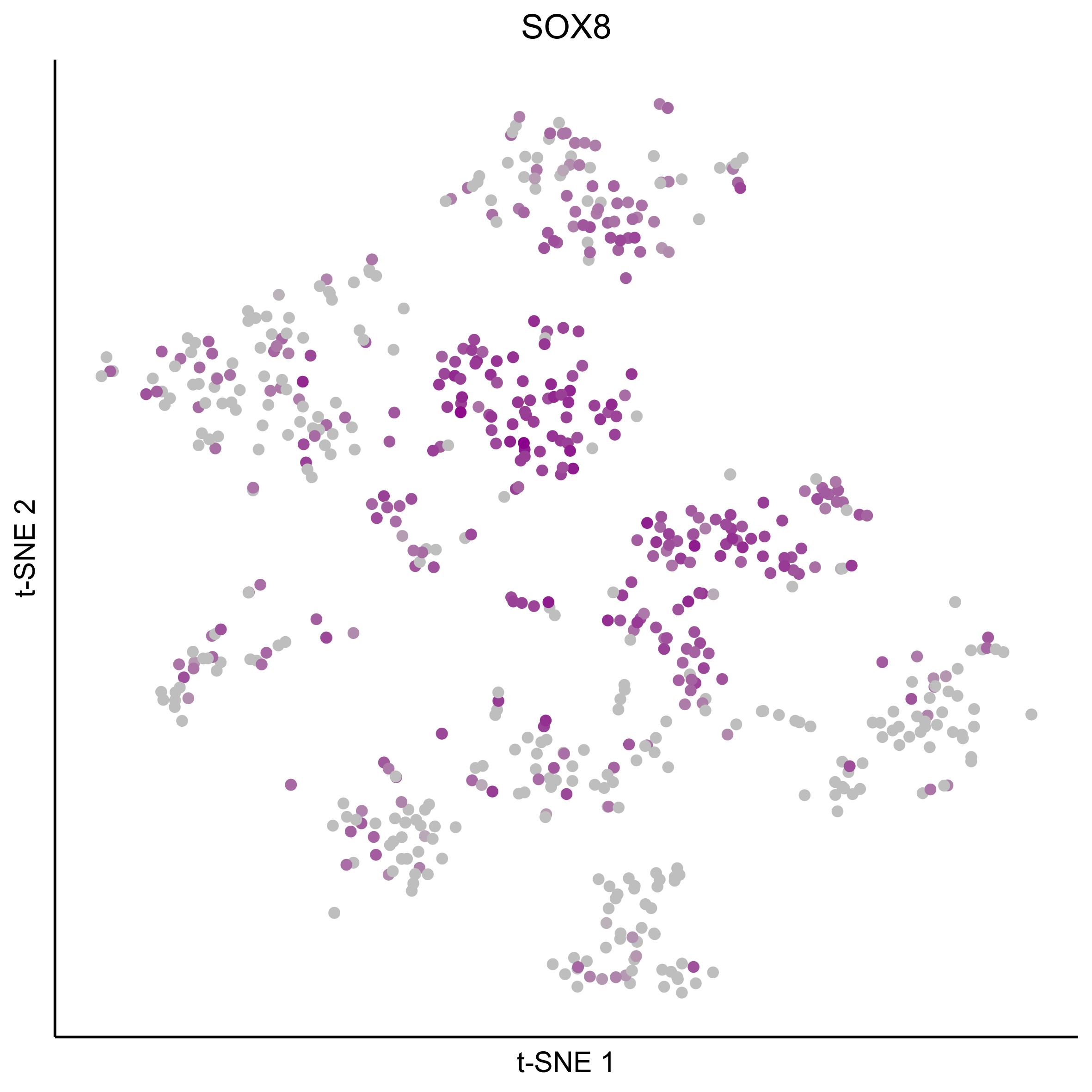
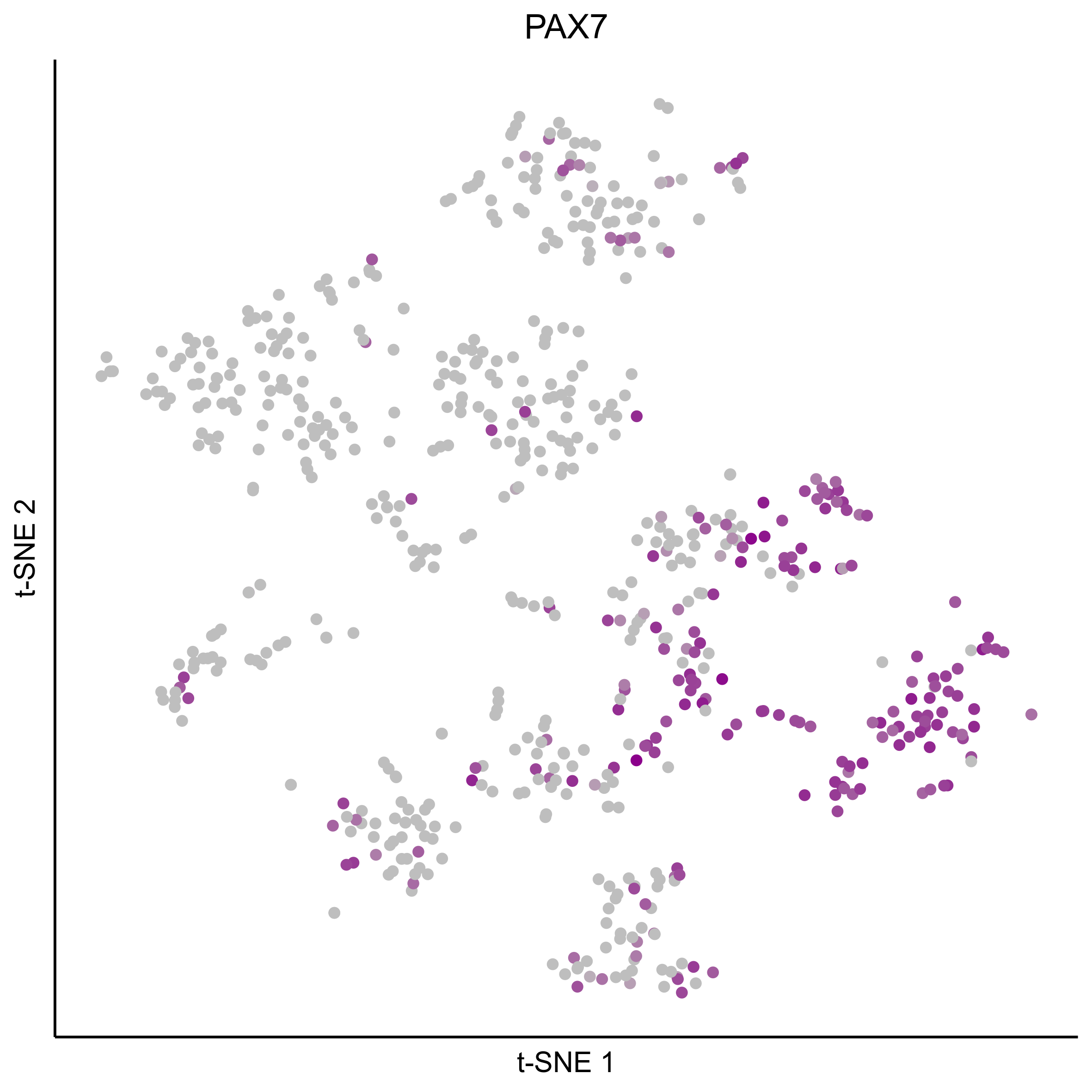
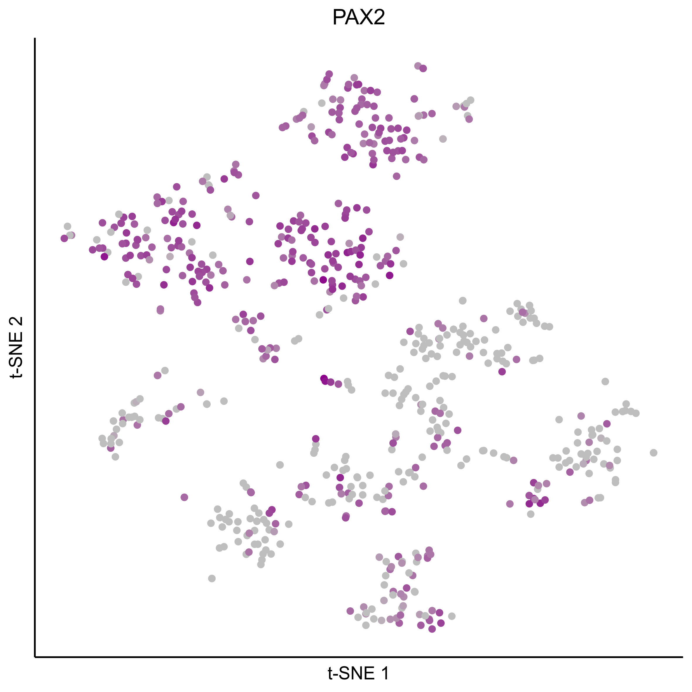
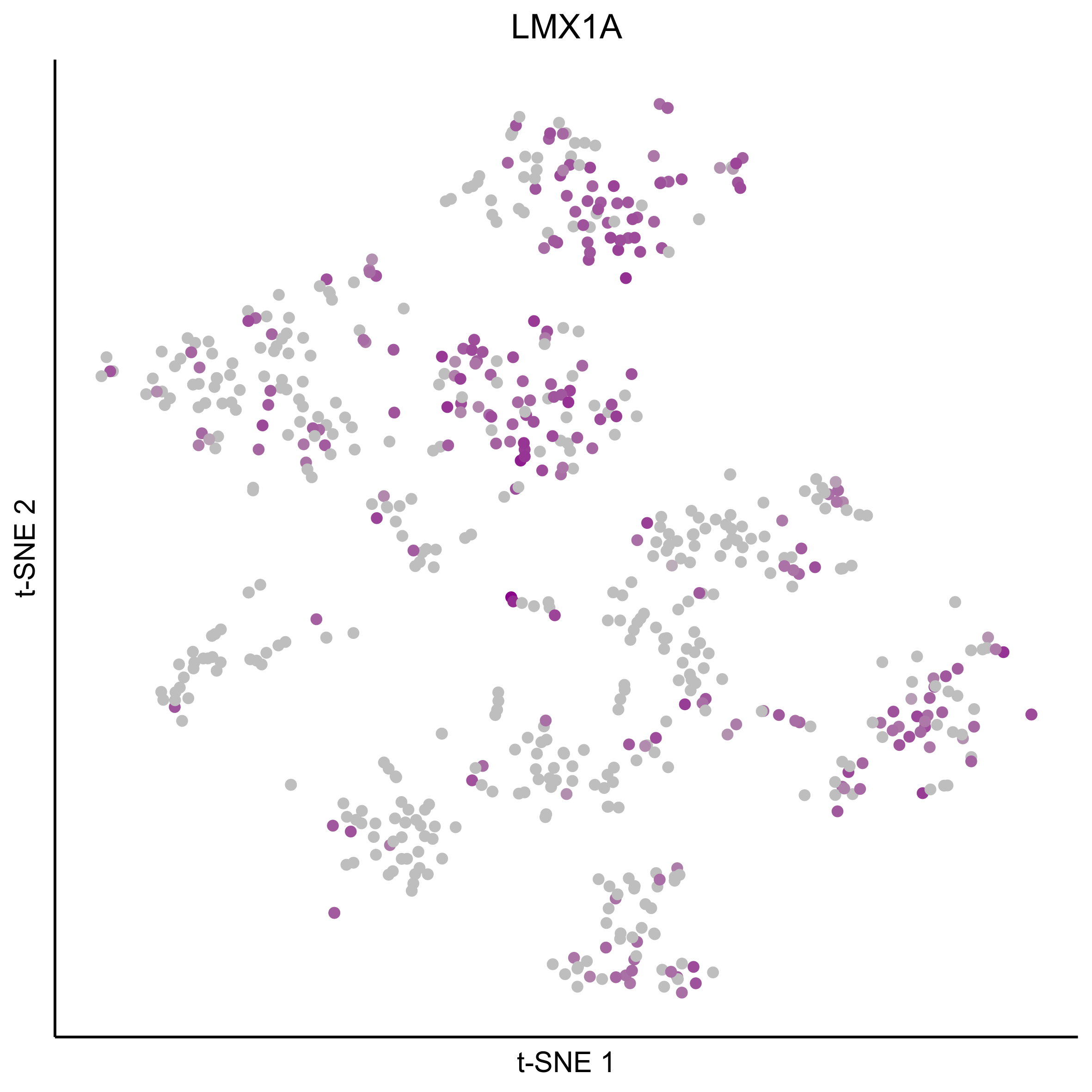
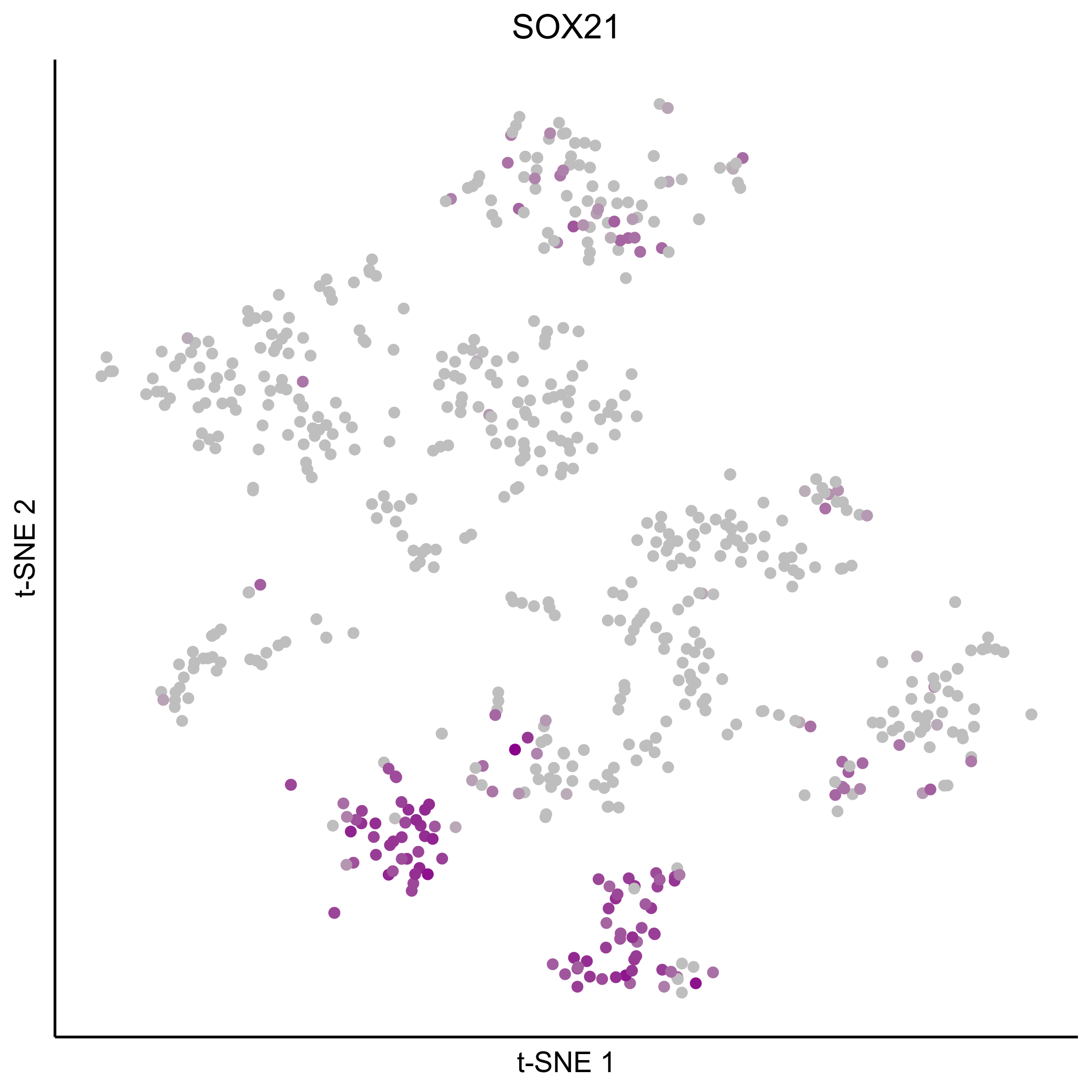
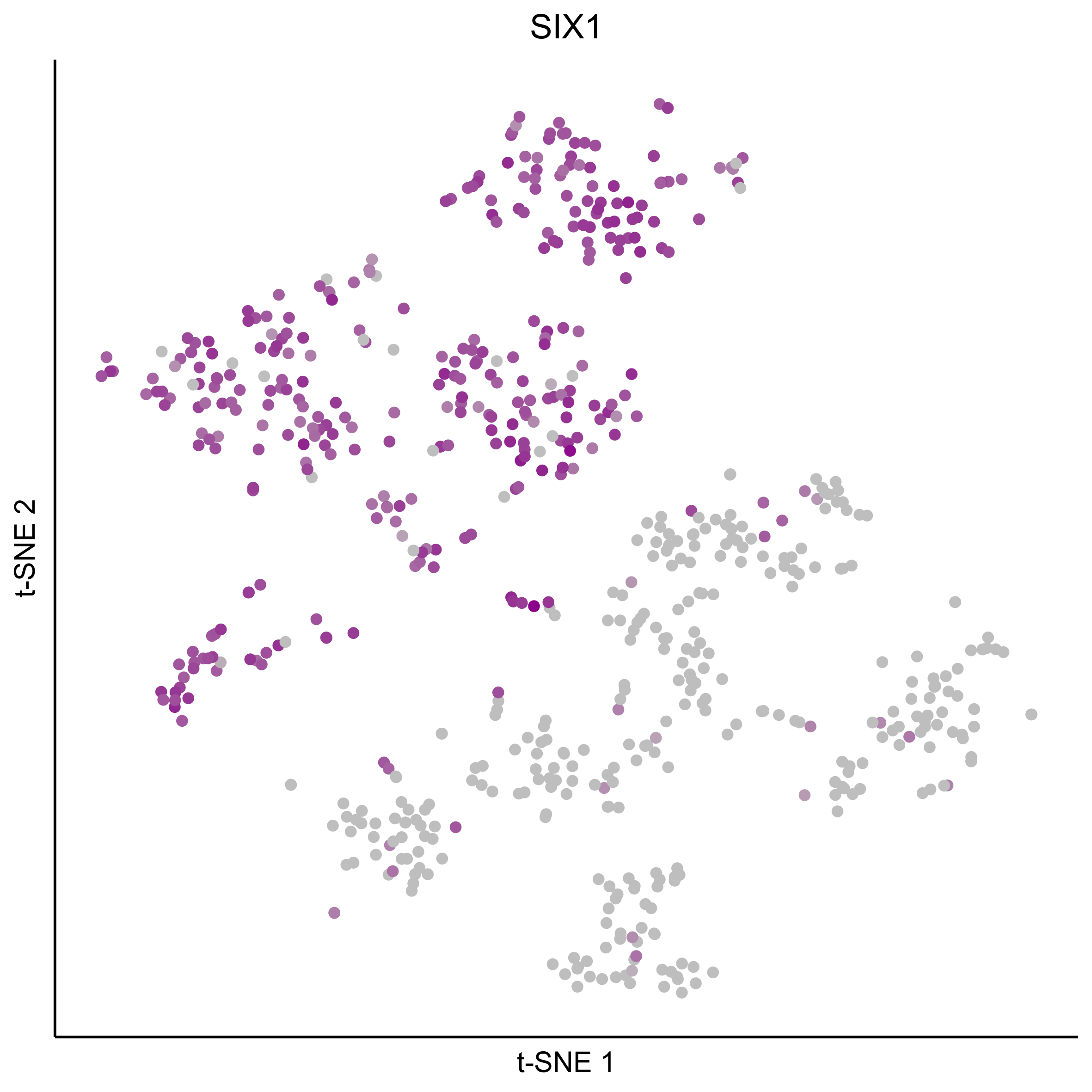
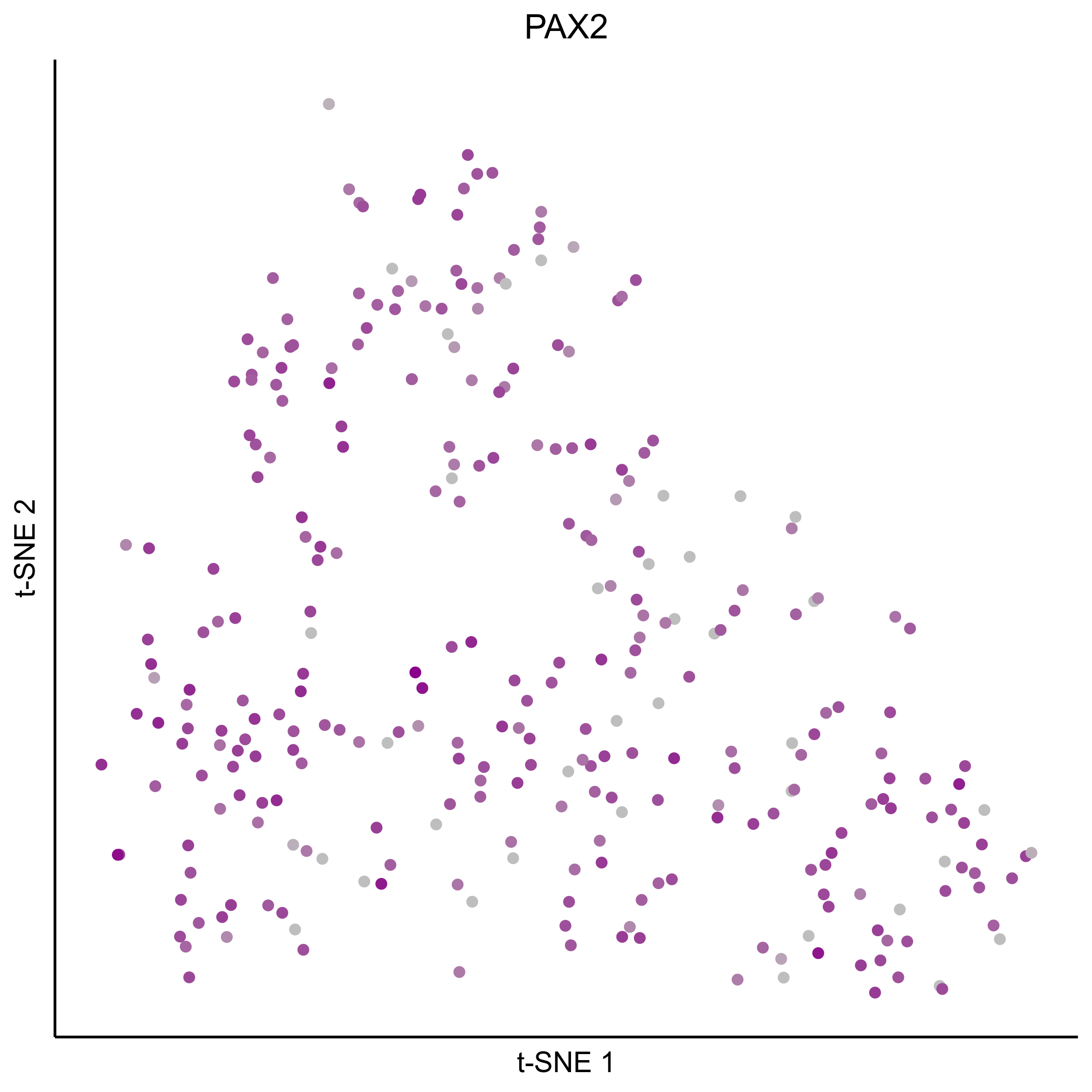
Plot tSNEs for genes of interest.
gene_list = c('SOX2', 'SOX10', 'SOX8', 'PAX7', 'PAX2', 'LMX1A', 'SOX21', 'SIX1')
for(gn in gene_list){
png(paste0(curr_plot_folder, gn, '_TSNE.png'), height = 15, width = 15, family = 'Arial', units = 'cm', res = 400)
print(tsne_plot(m2, m2$dR$genemodules, seed=seed, colour_by = as.integer(1+100*log10(1+m2$getReadcounts(data_status='Normalized')[gn,]) / max(log10(1+m2$getReadcounts(data_status='Normalized')[gn,]))),
colours = c("grey", "darkmagenta"), perplexity=perp, eta=eta) +
ggtitle(gn) +
theme(plot.title = element_text(hjust = 0.5)))
graphics.off()
}
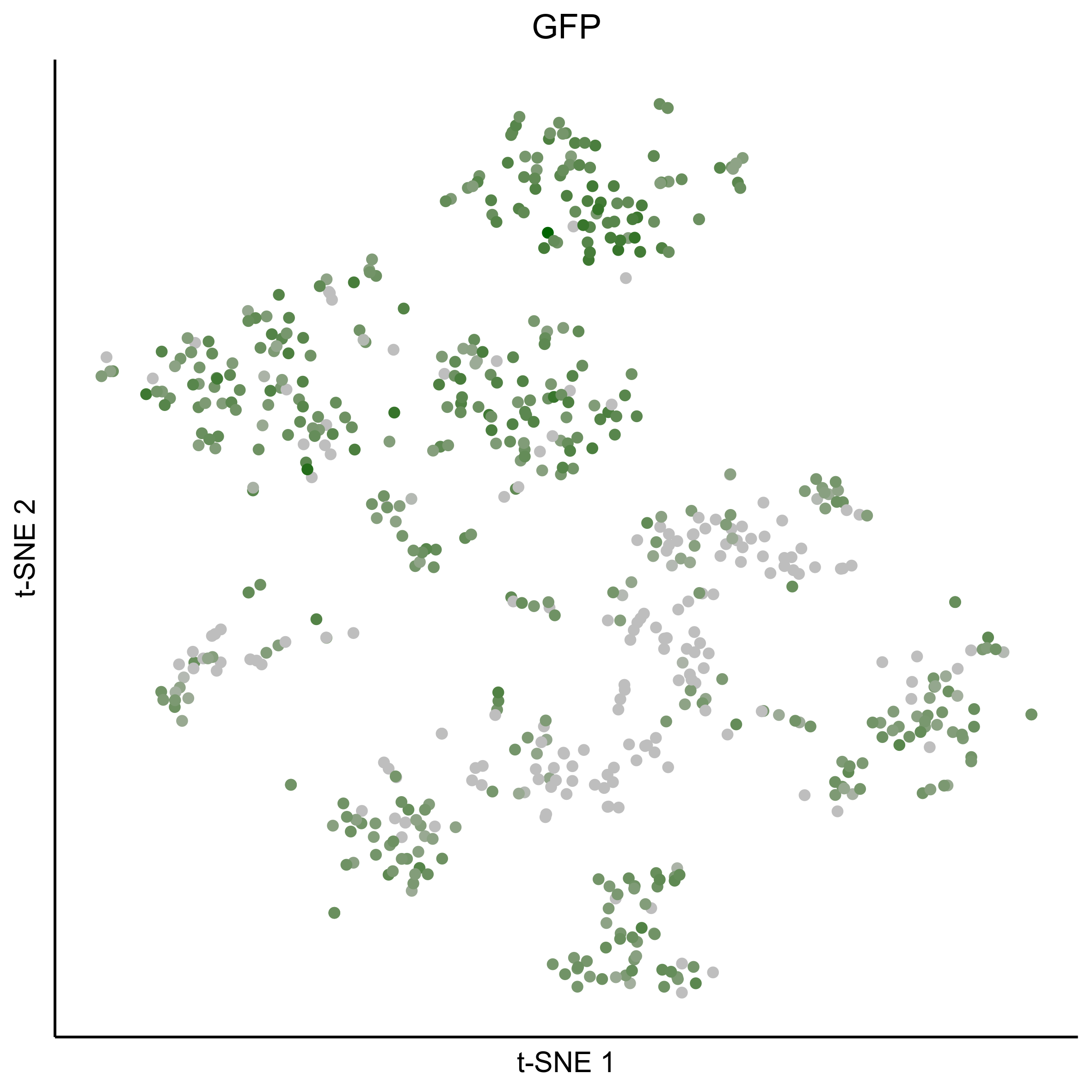
png(paste0(curr_plot_folder, 'GFP_TSNE.png'), height = 15, width = 15, family = 'Arial', units = 'cm', res = 400)
tsne_plot(m2, m2$dR$genemodules, seed=seed, colour_by = as.integer(1+100*log10(1+gfp_counts[m2$getCellsNames()]) / max(log10(1+gfp_counts[m2$getCellsNames()]))),
colours = c("grey", "darkgreen"), perplexity=perp, eta=eta) +
ggtitle('GFP') +
theme(plot.title = element_text(hjust = 0.5))
graphics.off()
Plot dotplot for genes of interest.
curr_plot_folder = paste0(plot_path, "all_cells/")
# gene list for dotplot
gene_list = c("DLX6", "HOMER2", "FOXI3", "TFAP2E", "ZNF385C", "SIX1", "PAX2", "DLX3", "NELL1", "FGF8", "VGLL2", "EYA1", "SOHO-1", "LMX1A", "SOX8", "ZBTB16", "DLX5", "TFAP2A", # Placodes
              "SOX10", "WNT1", "MSX2", "BMP5", "PAX7", "TFAP2B", "LMO4", "ETS1", "MSX1", "SOX9", # NC
              "ZEB2", "HOXA2", "SOX2", "RFX4", "PAX6", "WNT4", "SOX21", # Neural
              "SIM1", "PITX2", "TWIST1") # Mesoderm

# get cell branch information for dotplot
cell_cluster_data = data.frame(cluster = m2$cellClusters$Mansel$cell_ids) %>%
  tibble::rownames_to_column('cellname') %>%
  dplyr::mutate(celltype = case_when(
    cluster == "1" ~ "OEP",
    cluster == "2" ~ "Late Placodal",
    cluster == "3" ~ 'Neural',
    cluster == "4" ~ 'Mesodermal',
    cluster == "5" ~ 'Neural Crest'
  ))

# gather data for dotplot
dotplot_data <- data.frame(t(m2$getReadcounts('Normalized')[gene_list, ]), check.names=F) %>%
  tibble::rownames_to_column('cellname') %>%
  tidyr::gather(genename, value, -cellname) %>%
  dplyr::left_join(cell_cluster_data, by="cellname") %>%
  dplyr::group_by(genename, celltype) %>%
  # calculate percentage of cells in each cluster expressing gene
  dplyr::mutate('Proportion of Cells Expressing' = sum(value > 0)/n()) %>%
  # scale data
  dplyr::group_by(genename) %>%
  dplyr::mutate(value = scale(value)) %>%
  # calculate mean expression
  dplyr::group_by(genename, celltype) %>%
  dplyr::mutate('Scaled Average Expression'=mean(value)) %>%
  dplyr::distinct(genename, celltype, .keep_all=TRUE) %>%
  dplyr::ungroup() %>%
  # make factor levels to order genes in dotplot
  dplyr::mutate(genename = factor(genename, levels = gene_list)) %>%
  # make factor levels to order cells in dotplott
  dplyr::mutate(celltype = factor(celltype, levels = rev(c("OEP", "Late Placodal", "Neural Crest", "Neural", "Mesodermal"))))

png(paste0(curr_plot_folder, "all_cells_dotplot.png"), width=25, height=10, family = 'Arial', units = "cm", res = 400)
ggplot(dotplot_data, aes(x=genename, y=celltype, size=`Proportion of Cells Expressing`, color=`Scaled Average Expression`)) +
  geom_count() +
  scale_size_area(max_size=5) +
  scale_x_discrete(position = "top") + xlab("") + ylab("") +
  scale_color_gradient(low = "grey90", high = "blue") +
  theme_classic() +
  theme(axis.text.x = element_text(angle = 45, hjust = 0, size=9), axis.text.y = element_text(colour = clust.colors[c(4,3,5,2,1)], face = 'bold', size = 12),
        legend.position="bottom", legend.box = "horizontal", plot.margin=unit(c(0,1,0,0),"cm"))
graphics.off()
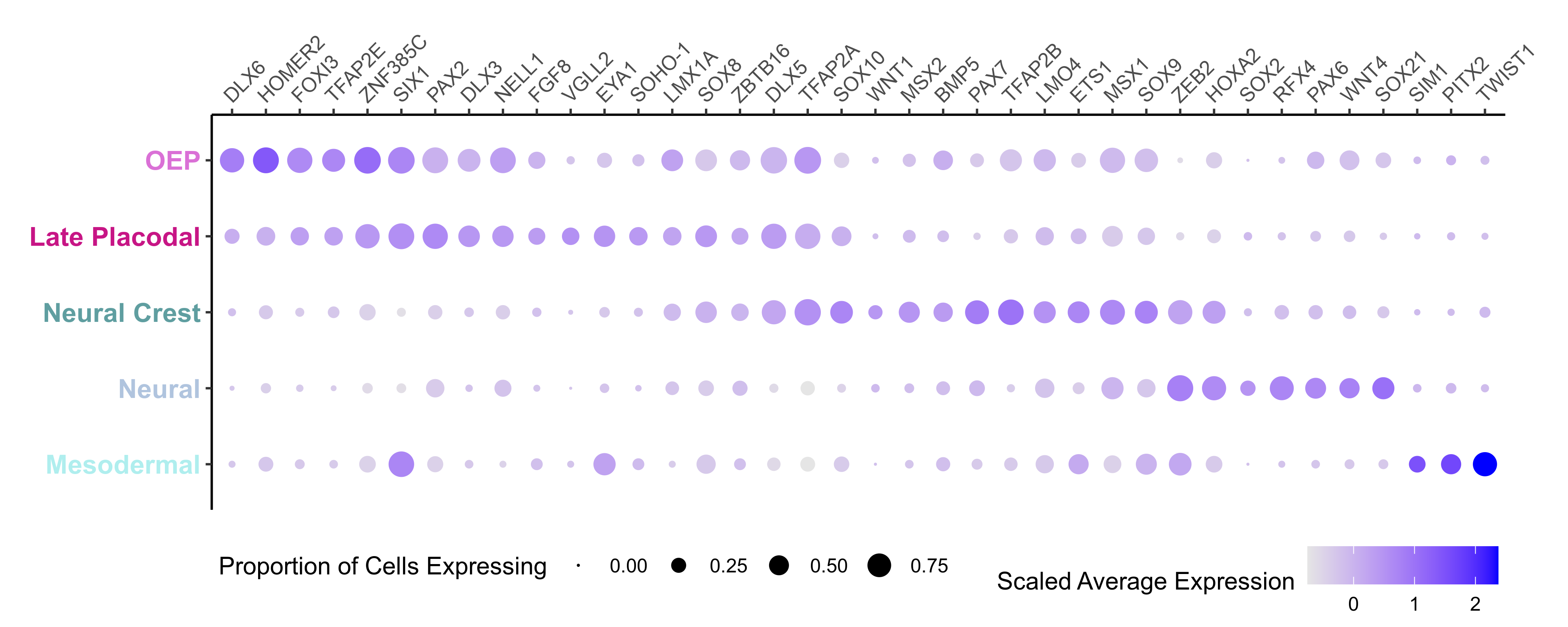
Clusters 3-5 are composed of non-oep derived populations (they are also mostly Pax2 negative).
We exclude these cells from the subsequent analysis.
curr_plot_folder = paste0(plot_path, "oep_subset/")
dir.create(curr_plot_folder)

m_oep = m2$copy()
m_oep$excludeCellFromClusterIds(cluster_ids=c(3:5), used_clusters='Mansel', data_status='Normalized')

#' Some genes may not be expressed any more in the remaining cells
m_oep$excludeUnexpressedGenes(min.cells=1, data_status="Normalized", verbose=TRUE)
m_oep$removeLowlyExpressedGenes(expression_threshold=1, selection_theshold=10, data_status='Normalized')
Calculate and plot gene modules for OEPs.
# "fastCor" uses the tcrossprod function which by default relies on BLAS to speed up computation. This produces inconsistent result in precision depending on the version of BLAS being used.
# see "matprod" in https://stat.ethz.ch/R-manual/R-devel/library/base/html/options.html
corr.mat2 = fastCor(t(m_oep$getReadcounts(data_status='Normalized')), method="spearman")

m_oep$identifyGeneModules(
  method="TopCorr_DR",
  corr=corr.mat2,
  corr_t = 0.3,
  topcorr_mod_min_cell=0, # default
  topcorr_mod_consistency_thres=0.4, # default
  topcorr_mod_skewness_thres=-Inf, # default
  topcorr_min_cell_level=5,
  data_status='Normalized'
)

names(m_oep$topCorr_DR$genemodules) <- paste0("GM ", seq(length(m_oep$topCorr_DR$genemodules)))

m_oep$writeGeneModules(folder_path = curr_plot_folder, basename='OEP_allGms', gms='topCorr_DR.genemodules')

m_oep$identifyCellClusters(method='hclust', used_genes="topCorr_DR.genemodules", data_status='Normalized')

m_oep$plotGeneModules(
  curr_plot_folder = curr_plot_folder,
  basename='OEP_allGms',
  displayed.gms = 'topCorr_DR.genemodules',
  displayed.geneset=NA,
  use.dendrogram='hclust',
  display.clusters=NULL,
  file_settings=list(list(type='pdf', width=10, height=10)),
  data_status='Normalized',
  gene_transformations='logscaled',
  pretty.params=list("size_factor"=2, "ngenes_per_lines" = 8, "side.height.fraction"=0.15),
  display.legend = FALSE,
  extra_legend=list("text"=c('ss8-9', 'ss11-12', 'ss14-15'), "colors"=unname(stage_cols))
)
Select gene modules based on the presence of genes known to be involved in Otic and Epibranchial development and re-cluster cells.
bait_genes = c("HOMER2", "LMX1A", "SOHO-1", "SOX10", "VGLL2", "FOXI3", 'ZNF385C', 'NELL1', "CXCL14", "EYA4")

m_oep$topCorr_DR$genemodules.selected = Filter(function(x){any(bait_genes %in% x)}, m_oep$topCorr_DR$genemodules)

# cluster into 5 clusters
m_oep$identifyCellClusters(method='hclust', clust_name="Mansel", used_genes="topCorr_DR.genemodules.selected", data_status='Normalized', numclusters=5)

clust.colors <- c('#ffa07a', '#f55f20', '#dda0dd', '#48d1cc', '#b2ffe5')

m_oep$plotGeneModules(
  curr_plot_folder = curr_plot_folder,
  basename='OEP_GMselection',
  displayed.gms = 'topCorr_DR.genemodules.selected',
  displayed.geneset=NA,
  use.dendrogram='Mansel',
  file_settings=list(list(type='pdf', width=10, height=5)),
  data_status='Normalized',
  gene_transformations=c('log', 'logscaled'),
  extra_colors=cbind(
    m_oep$cellClusters$Mansel$cell_ids %>% clust.colors[.]
  ),
  display.legend = FALSE,
  pretty.params=list("size_factor"=2, "ngenes_per_lines" = 6, "side.height.fraction"=0.5),
  extra_legend=list("text"=c('ss8-9', 'ss11-12', 'ss14-15'), "colors"=unname(stage_cols))
)

# add gene modules txt
m_oep$writeGeneModules(folder_path = curr_plot_folder, basename='OEP_GMselection', gms='topCorr_DR.genemodules')
Download gene module list - SuppData2
Plot tSNEs of cell clusters and developmental stage.
curr_plot_folder = paste0(plot_path, 'oep_subset/tsne/')
dir.create(curr_plot_folder)

png(paste0(curr_plot_folder, 'OEP_clusters_TSNE.png'), height = 15, width = 15, family = 'Arial', units = 'cm', res = 400)
tsne_plot(m_oep, m_oep$topCorr_DR$genemodules.selected, seed=seed, colour_by=m_oep$cellClusters[['Mansel']]$cell_ids, colours=clust.colors, perplexity=perp, eta=eta) +
ggtitle('Clusters') +
theme(plot.title = element_text(hjust = 0.5))
graphics.off()

png(paste0(curr_plot_folder, 'OEP_stage_TSNE.png'), height = 15, width = 15, family = 'Arial', units = 'cm', res = 400)
tsne_plot(m_oep, m_oep$topCorr_DR$genemodules.selected, seed=seed, colour_by = pData(m_oep$expressionSet)$timepoint, colours = stage_cols, perplexity=perp, eta=eta) +
ggtitle('Developmental stage') +
theme(plot.title = element_text(hjust = 0.5))
graphics.off()
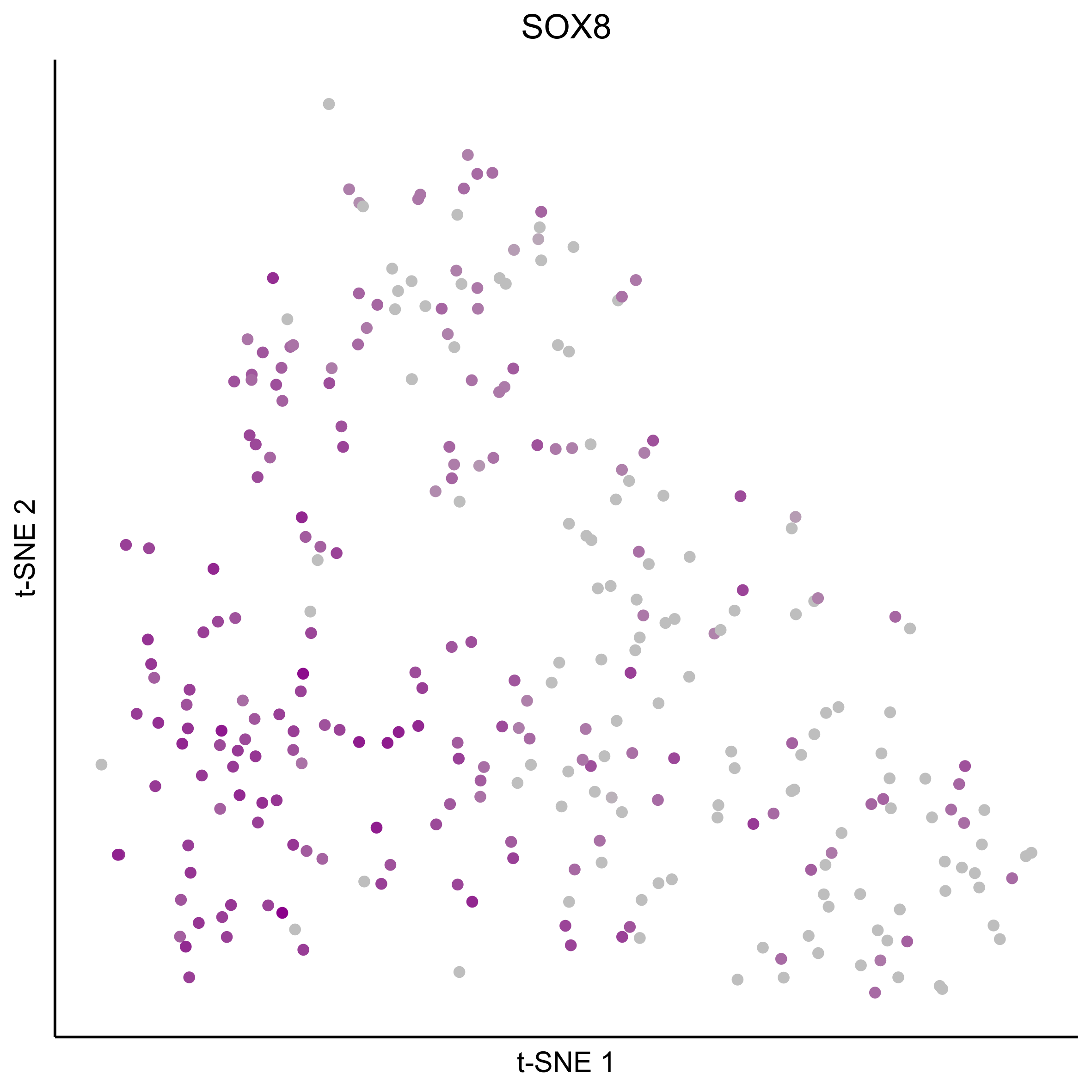
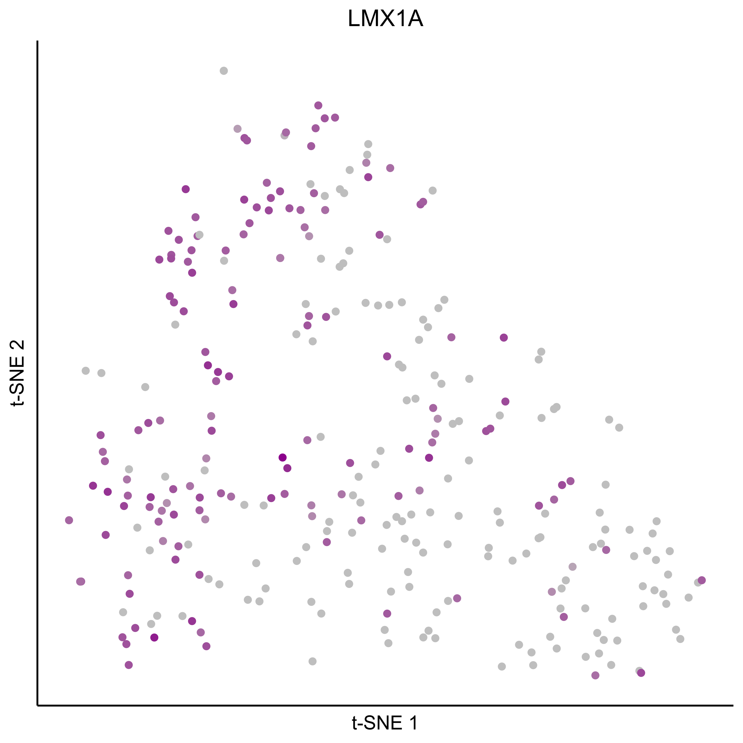
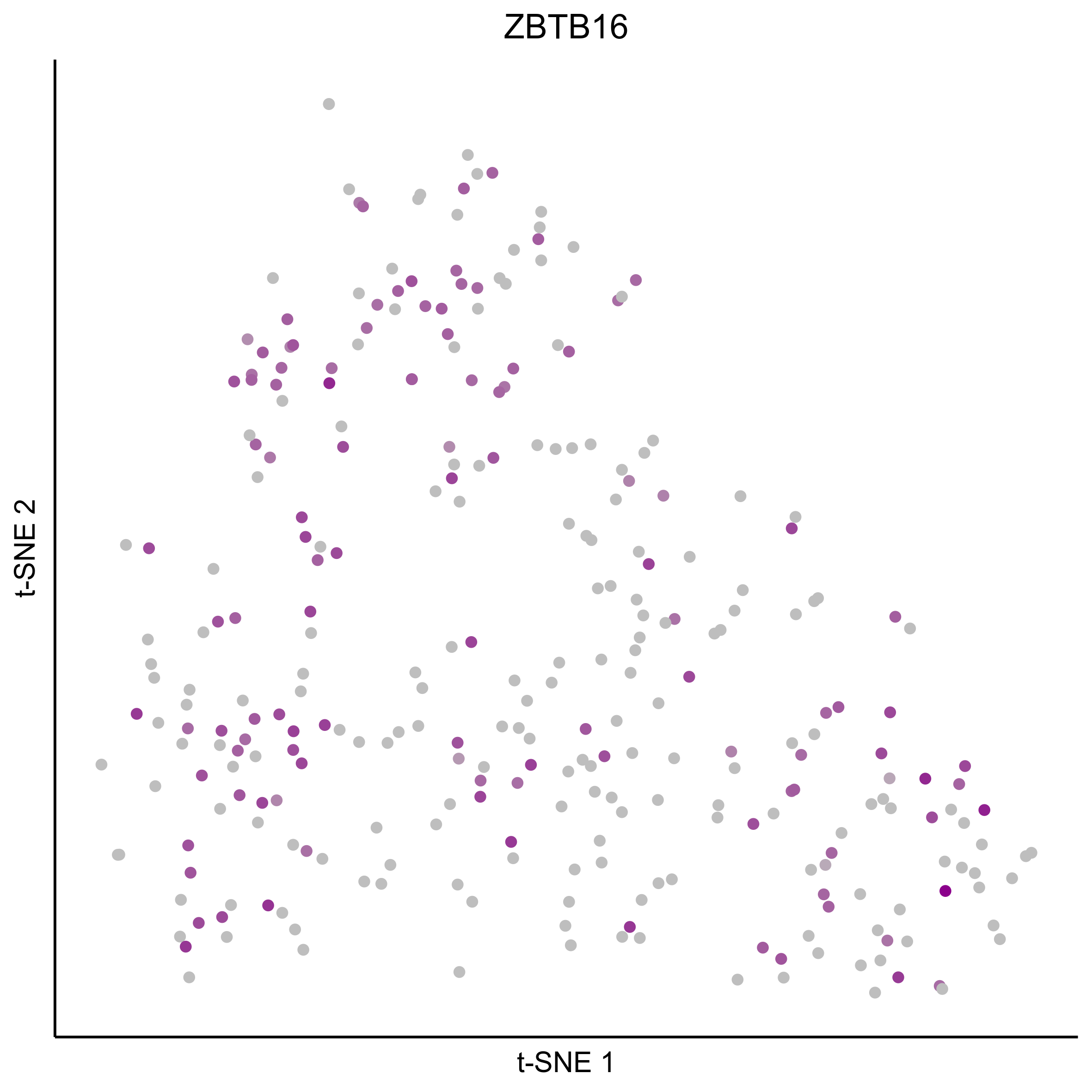
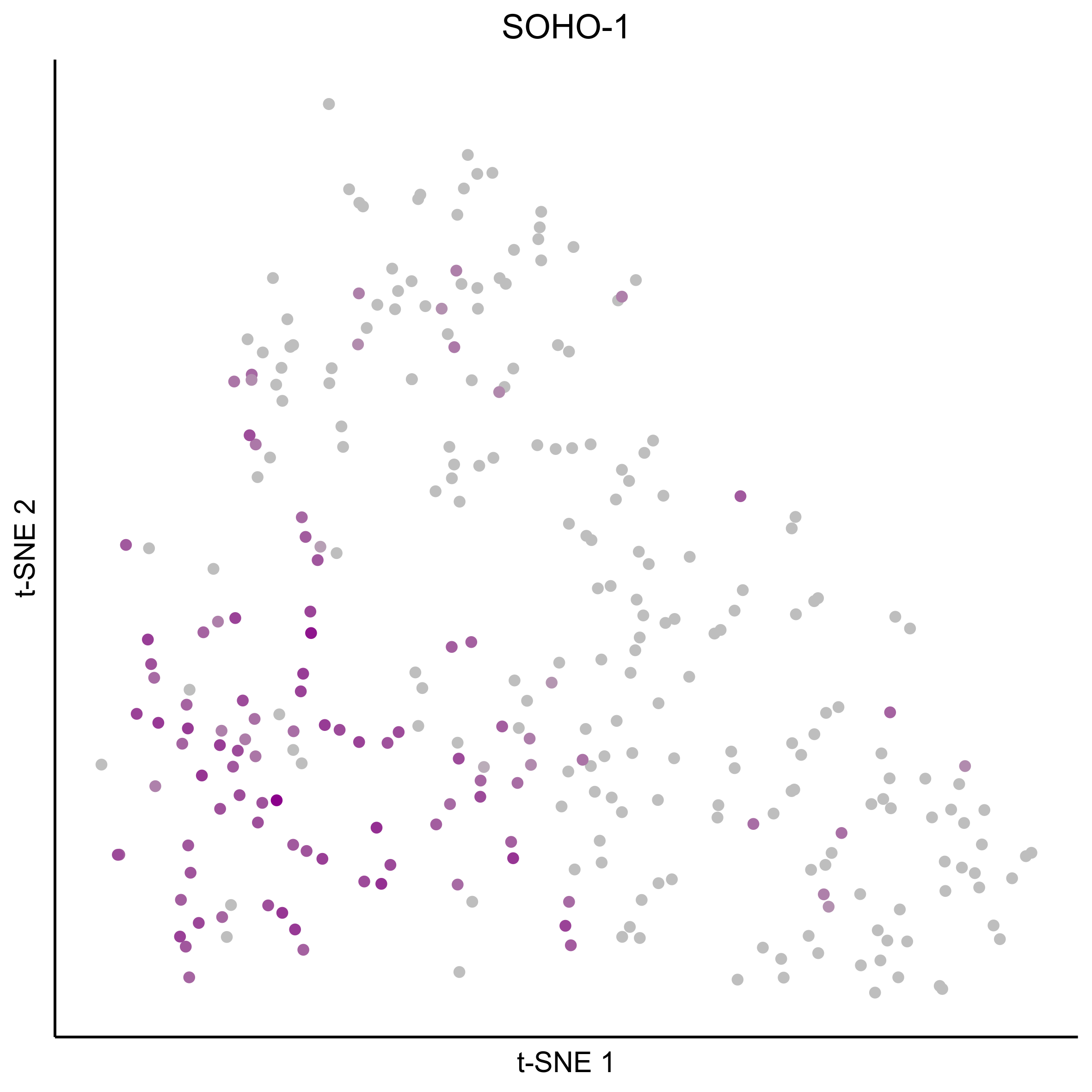
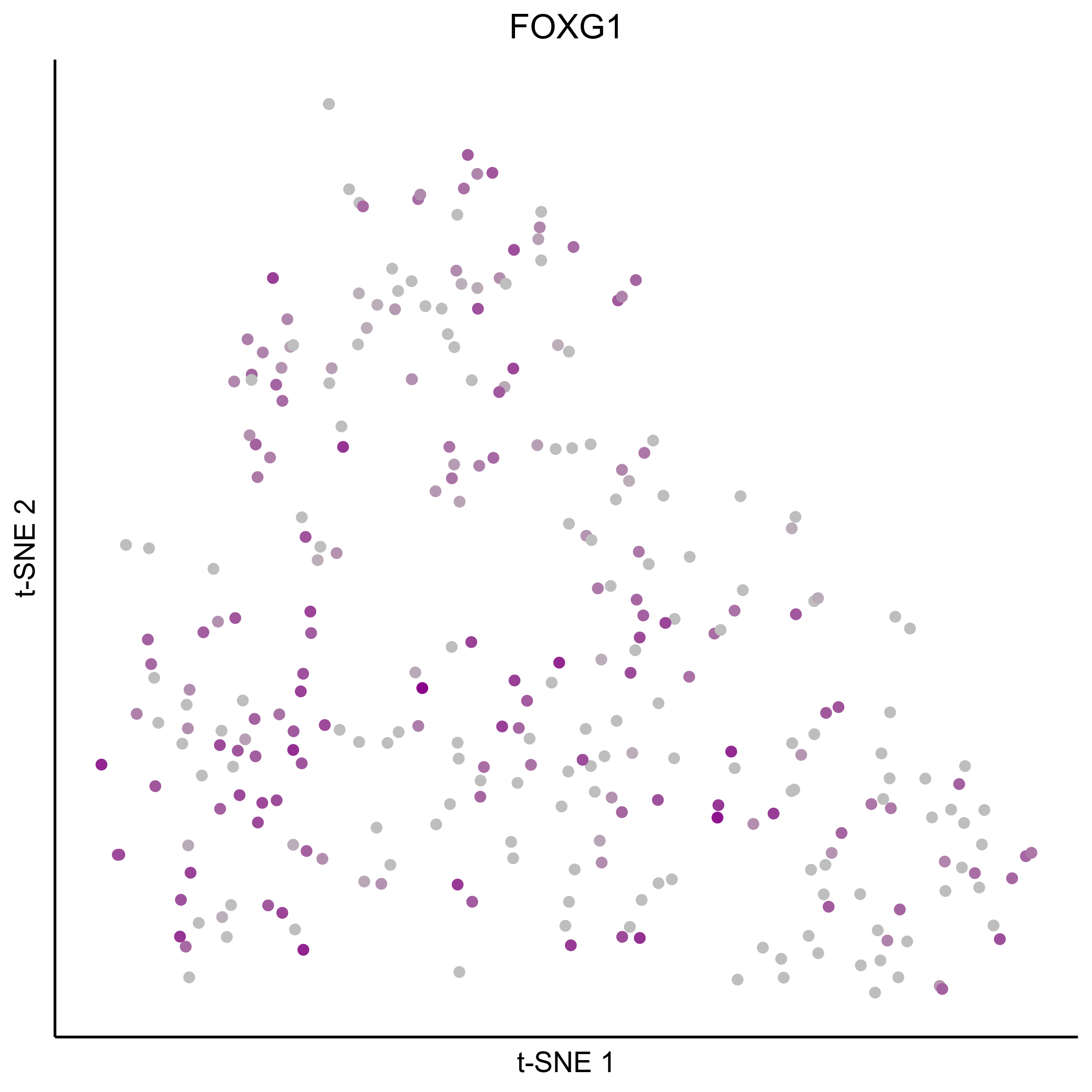
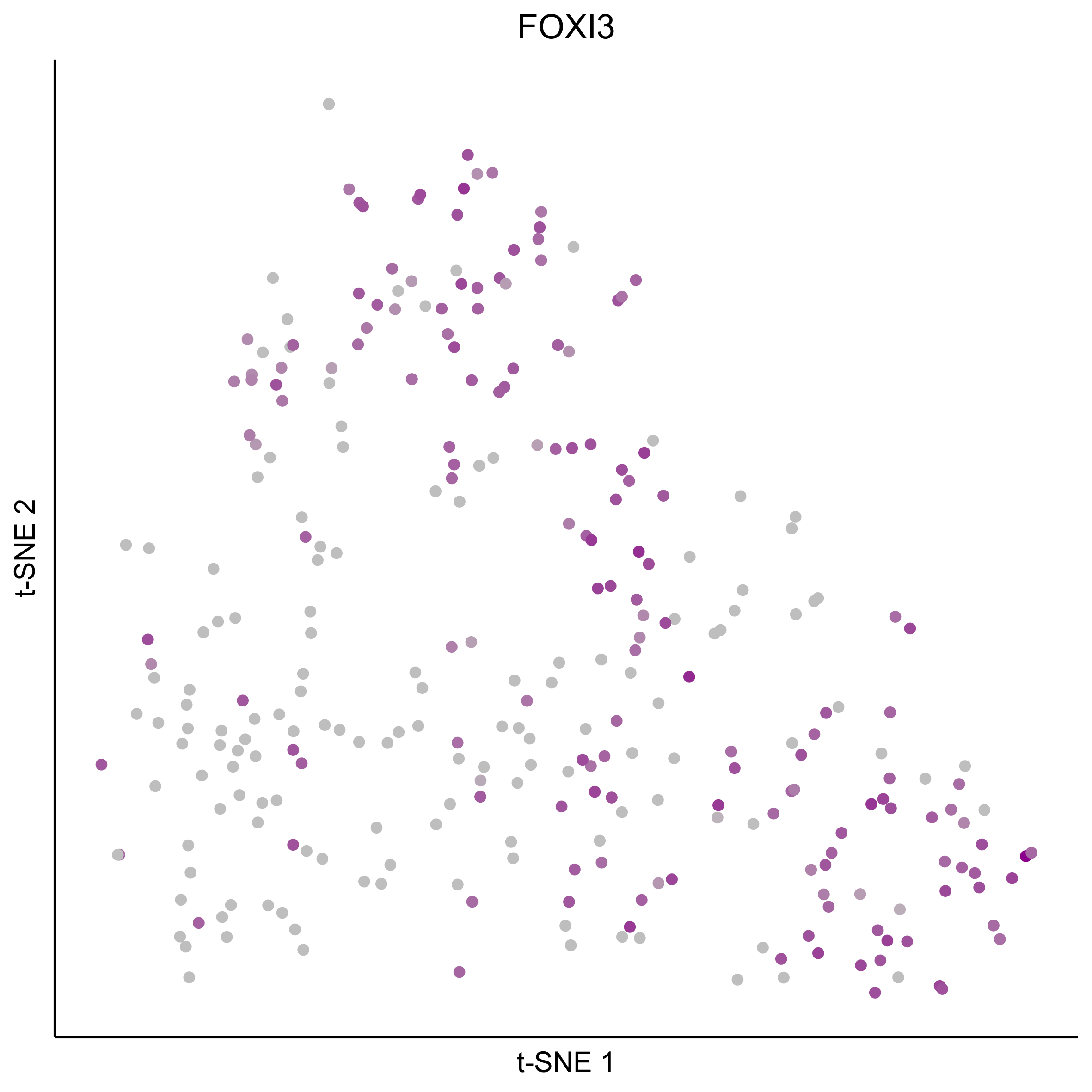
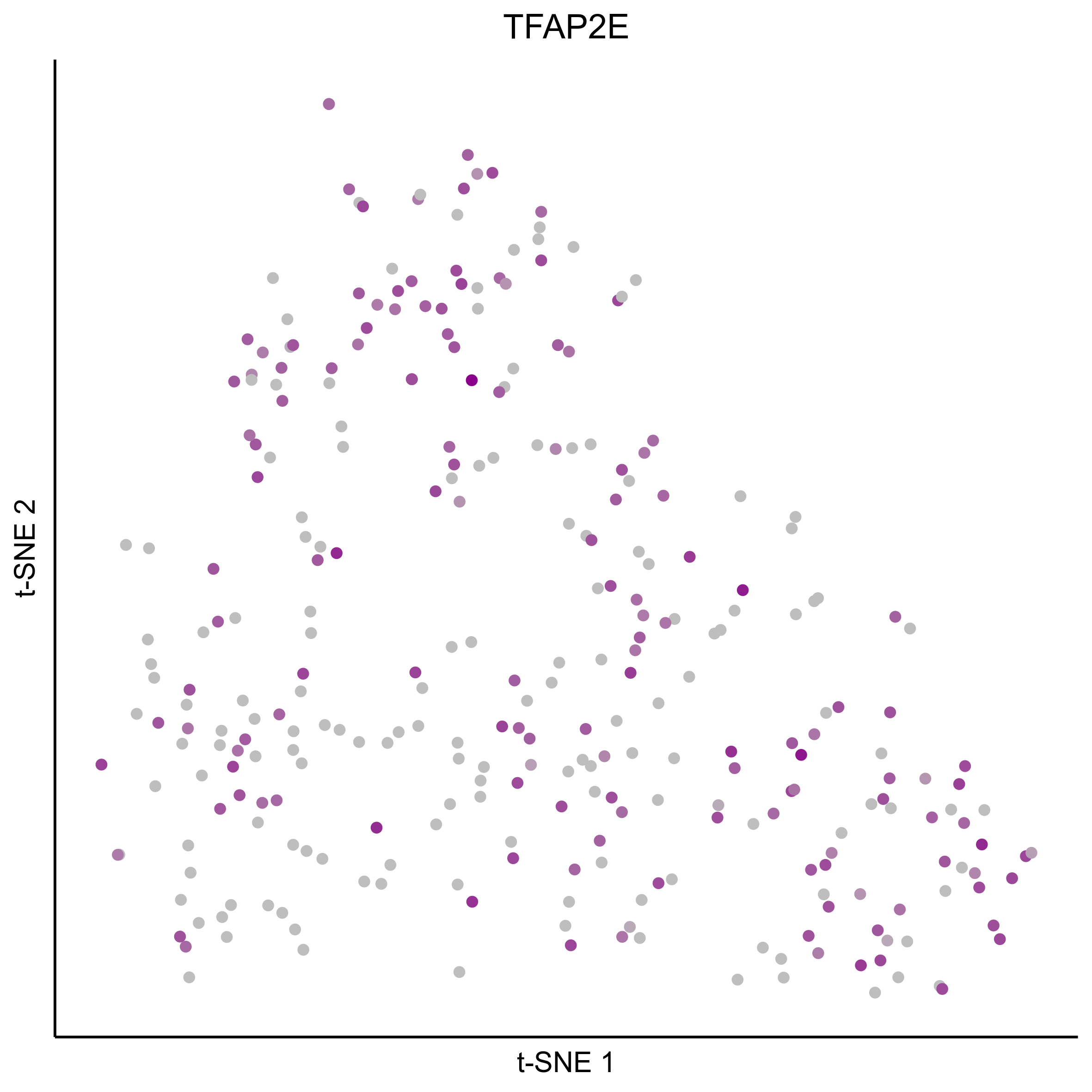
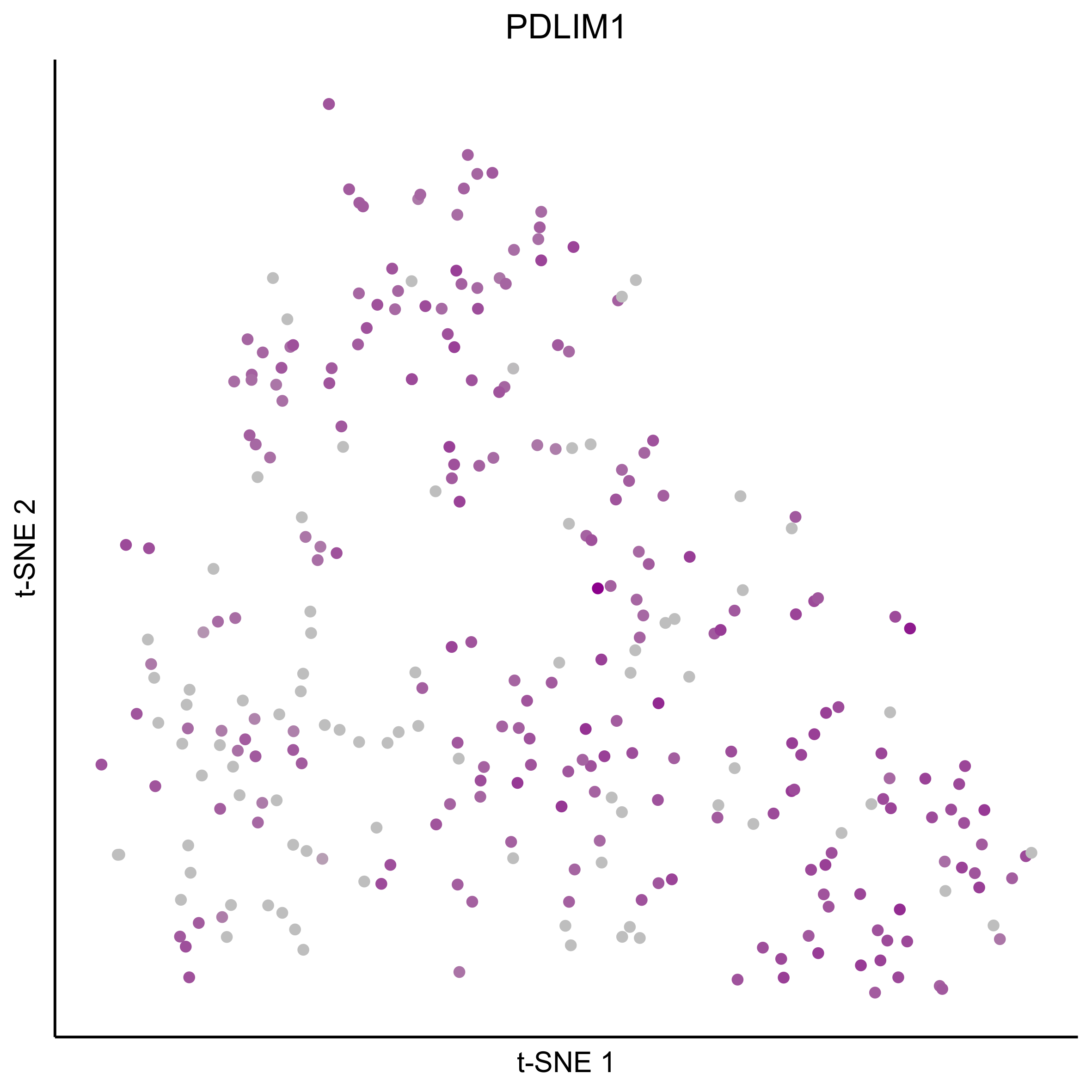
Plot tSNEs for bait genes, as well as genes from bulk RNAseq and from the literature.
gene_list = c(bait_genes, 'SOX8', 'PAX2', 'TFAP2E', 'SIX1', 'ZBTB16', 'FOXG1', 'PDLIM1')
for(gn in gene_list){
png(paste0(curr_plot_folder, gn, '\_TSNE.png'), height = 15, width = 15, family = 'Arial', units = 'cm', res = 400)
print(tsne_plot(m_oep, m_oep$topCorr_DR$genemodules.selected, seed=seed, colour_by = as.integer(1+100*log10(1+m_oep$getReadcounts(data_status='Normalized')[gn,]) / max(log10(1+m_oep$getReadcounts(data_status='Normalized')[gn,]))),
colours = c("grey", "darkmagenta"), perplexity=perp, eta=eta) +
ggtitle(gn) +
theme(plot.title = element_text(hjust = 0.5)))
graphics.off()
}
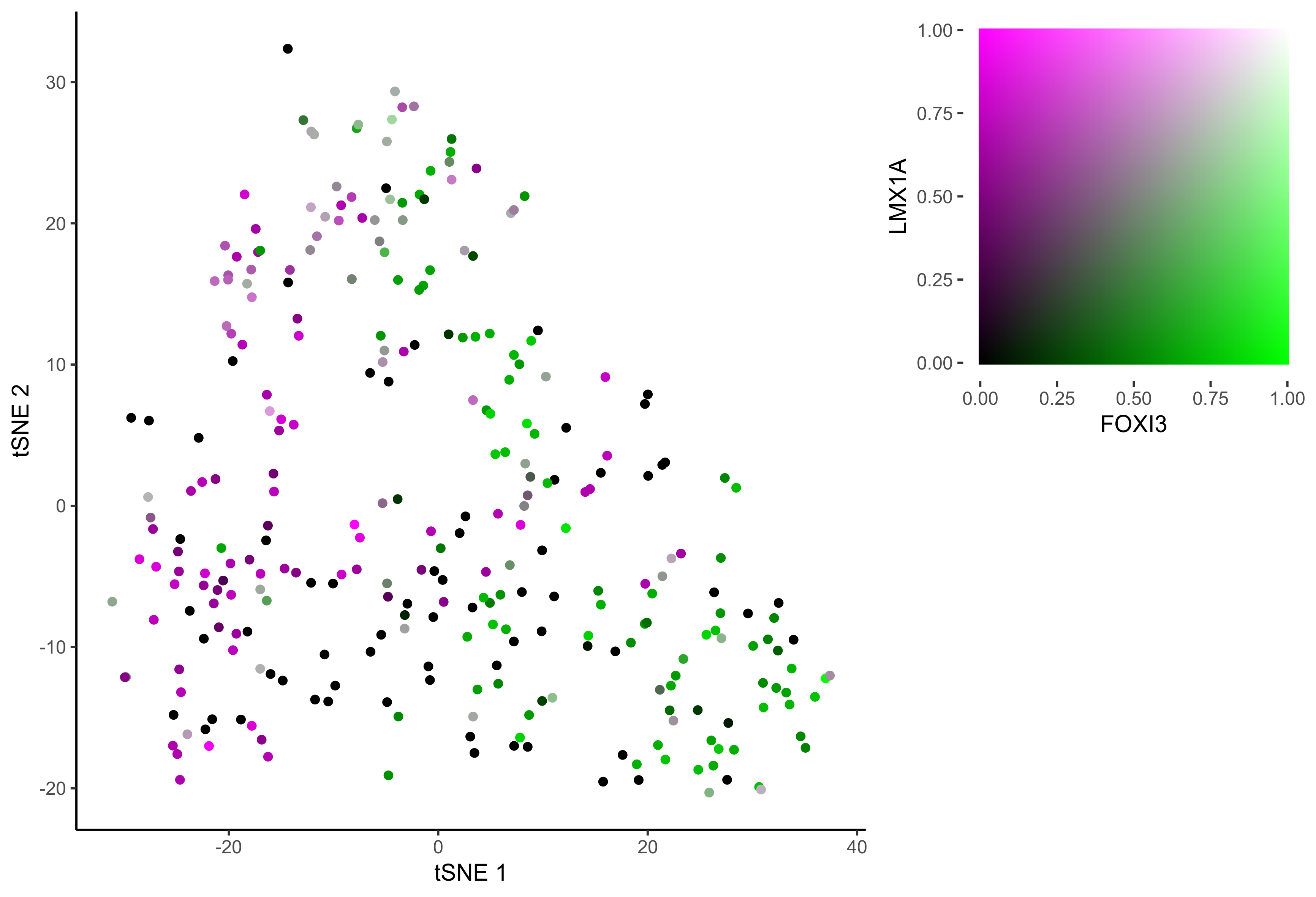
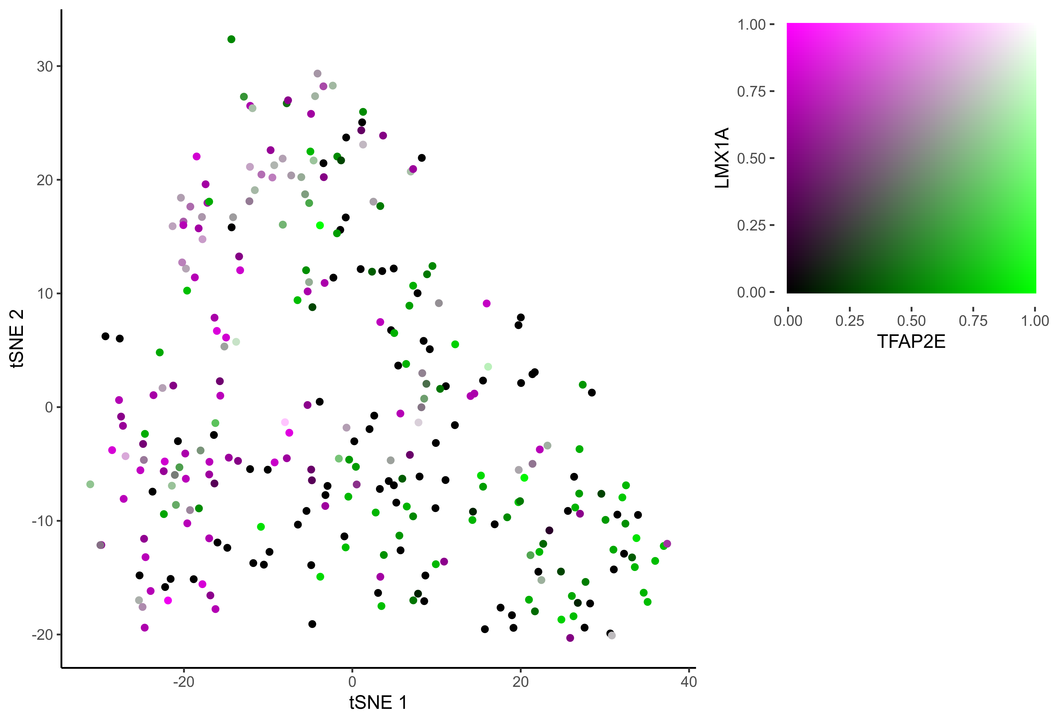
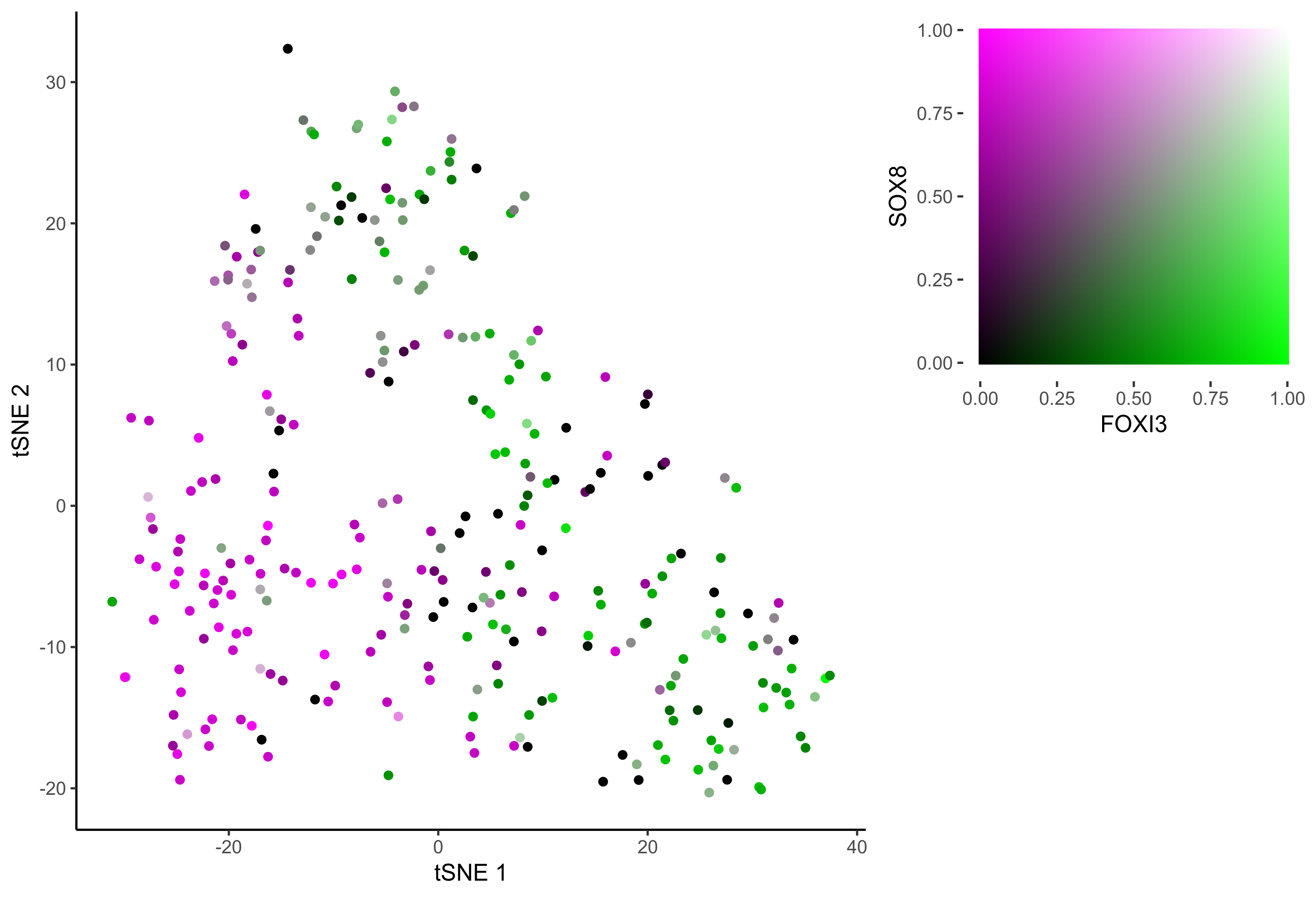
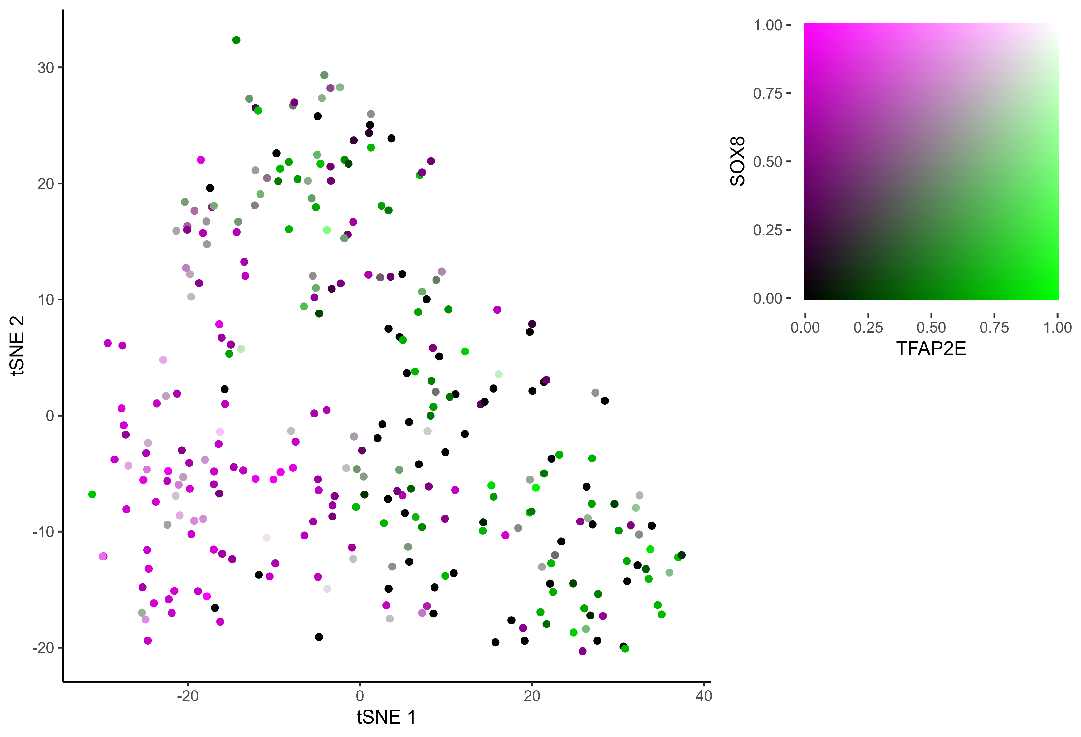
Plot tSNE co-expression plots.
gene_pairs <- list(c("FOXI3", "LMX1A"), c("TFAP2E", "LMX1A"), c("FOXI3", "SOX8"), c("TFAP2E", "SOX8"))
lapply(gene_pairs, function(x) {plot_tsne_coexpression(m_oep, m_oep$topCorr_DR$genemodules.selected, gene1 = x[1], gene2 = x[2], plot_folder = curr_plot_folder,
seed=seed, perplexity=perp, pca=FALSE, eta=eta, height = 15, width = 22, res = 400, units = 'cm', family = 'Arial')})
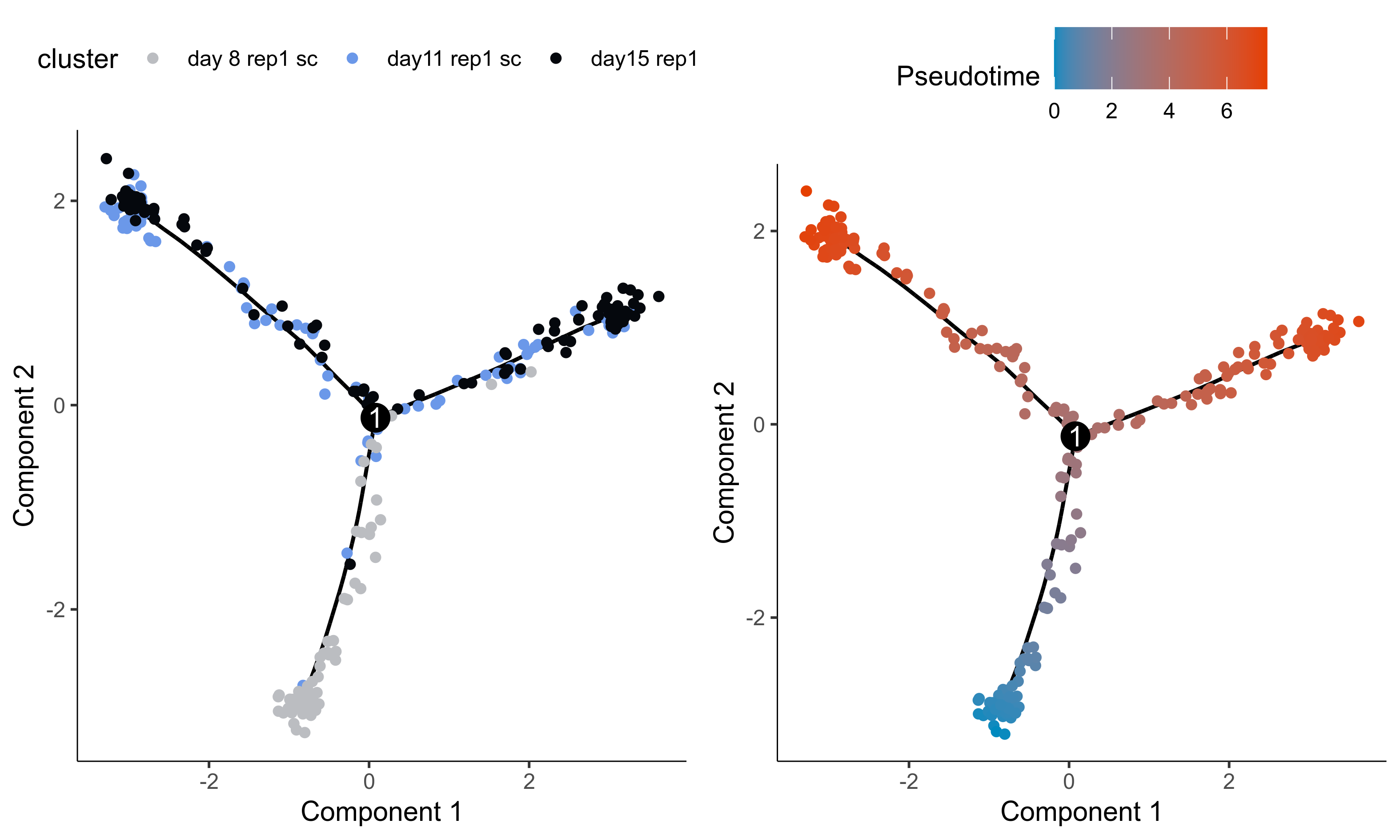
In order to study the process of differentiation from OEP to Otic and Epibranchial lineages, we order the cells in pseudotime.
curr_plot_folder = paste0(plot_path, "monocle_plots/")
dir.create(curr_plot_folder)

# gene modules for biological process of interest
monocle.input_dims = unlist(m_oep$topCorr_DR$genemodules.selected)

# input Antler data into Monocle
df_pheno = pData(m_oep$expressionSet)
df_feature = cbind(fData(m_oep$expressionSet), 'gene_short_name'=fData(m_oep$expressionSet)$current_gene_names) # "gene_short_name" may be required by monocle
rownames(df_feature) <- df_feature$gene_short_name

HSMM <- monocle::newCellDataSet(
  as.matrix(m_oep$getReadcounts(data_status='Normalized')),
  phenoData = new("AnnotatedDataFrame", data = df_pheno),
  featureData = new('AnnotatedDataFrame', data = df_feature),
  lowerDetectionLimit = .1,
  expressionFamily=VGAM::tobit()
)

# Dimensionality reduction and order cells along pseudotime
HSMM <- estimateSizeFactors(HSMM)
HSMM <- setOrderingFilter(HSMM, monocle.input_dims)
HSMM <- reduceDimension(HSMM, max_components = 2, method = 'DDRTree')
HSMM <- orderCells(HSMM)

# Root cells to earliest "State" (ie DDRTree branch) - which is stage 8
HSMM <- orderCells(HSMM, root_state = which.max(table(pData(HSMM)$State, pData(HSMM)$timepoint)[, "8"]))
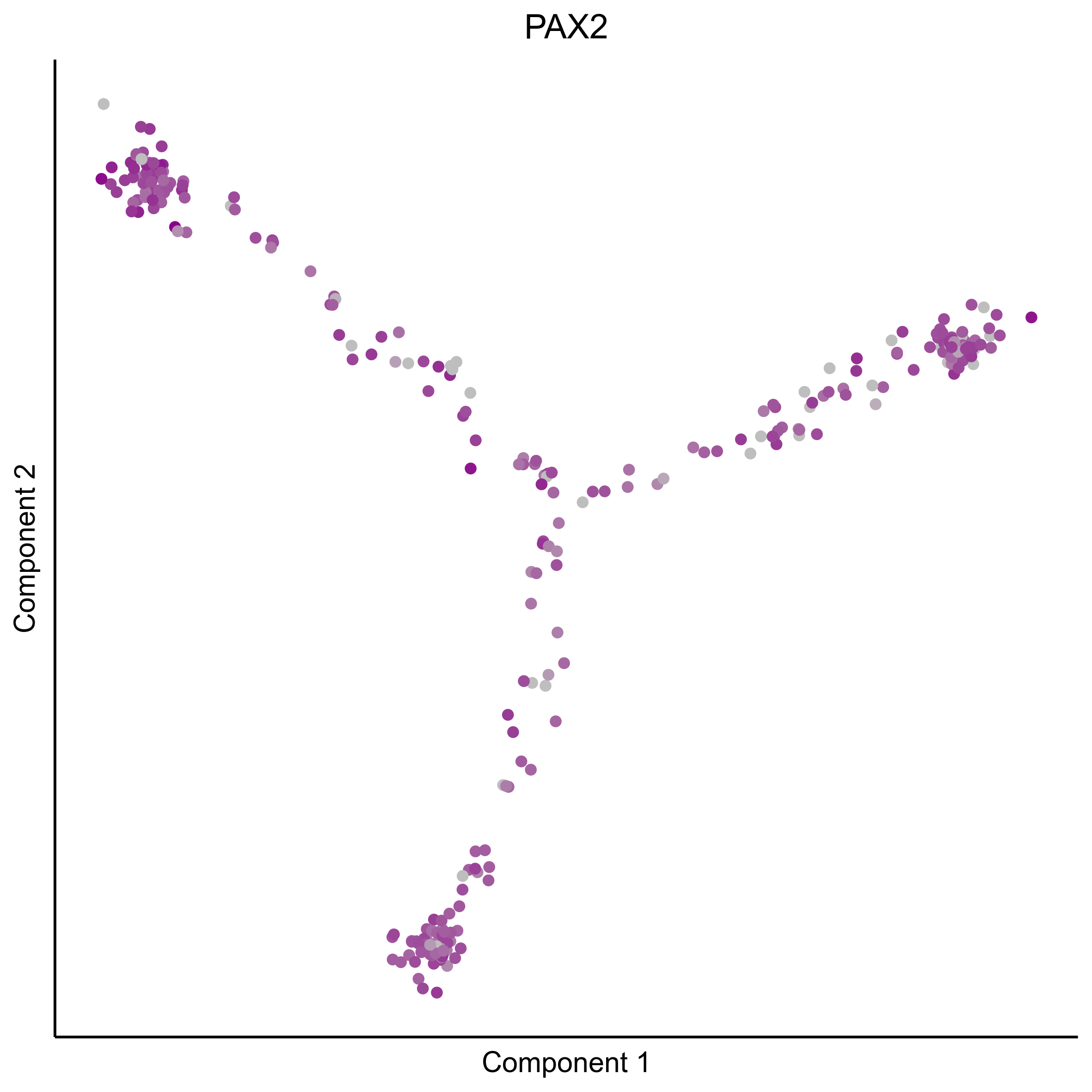
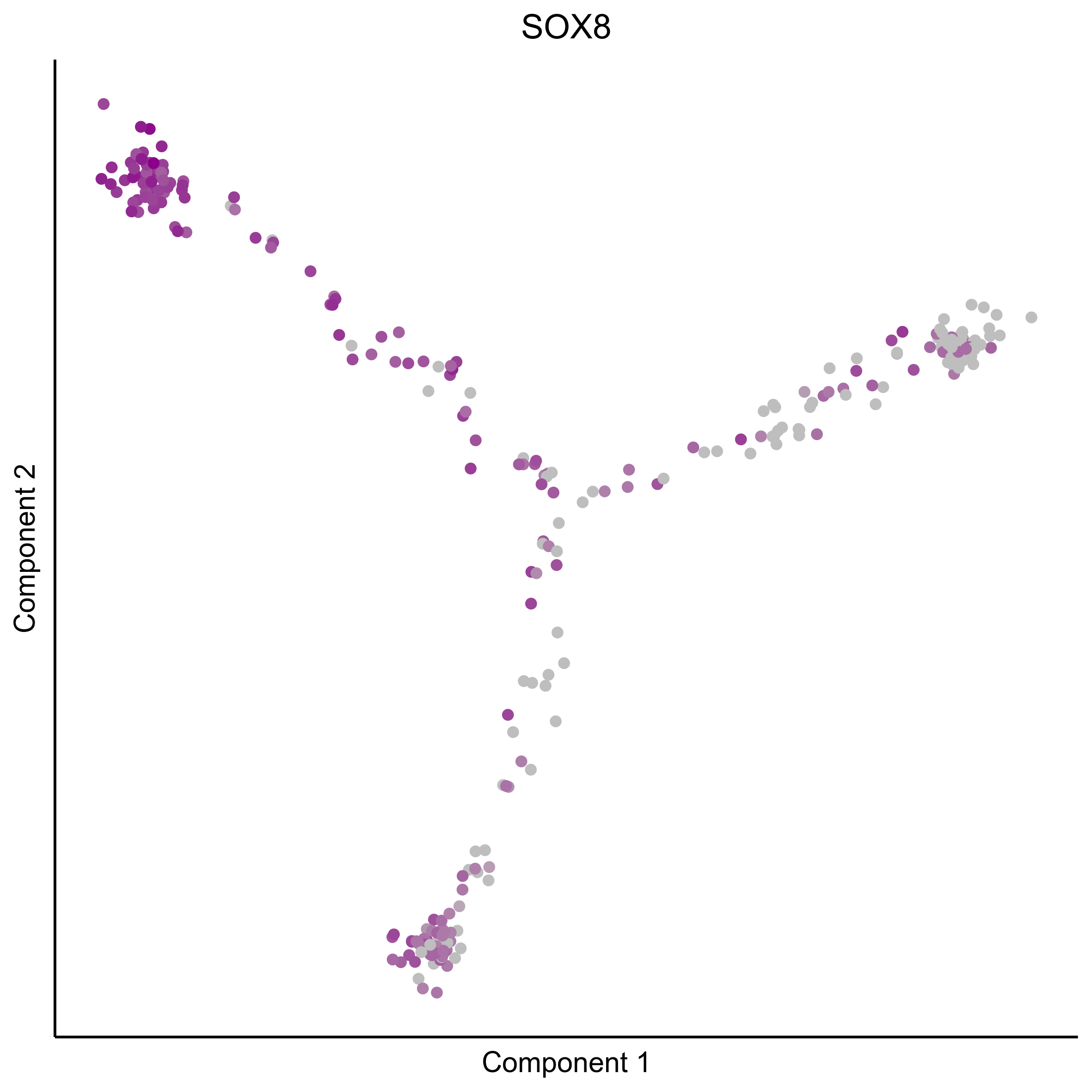
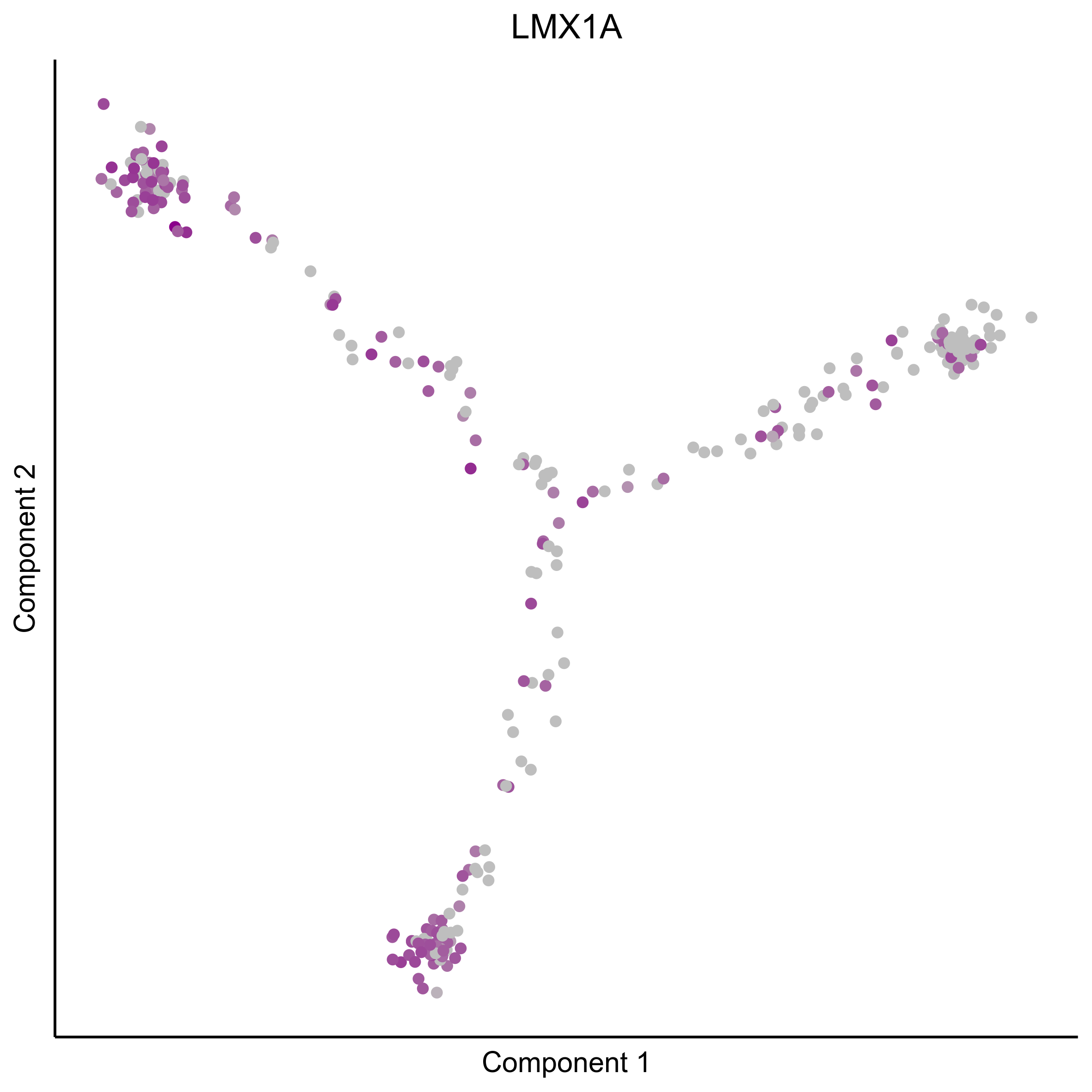
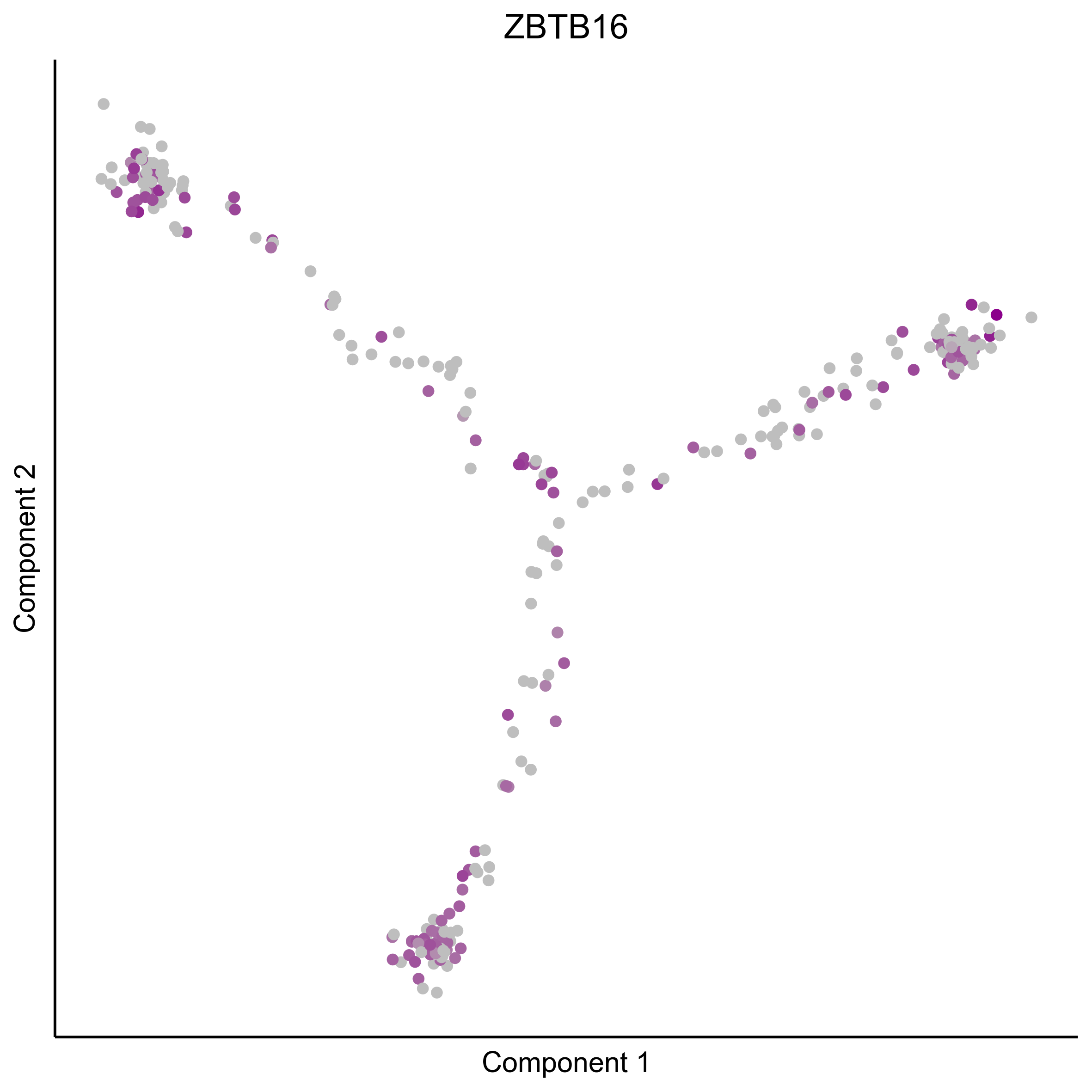
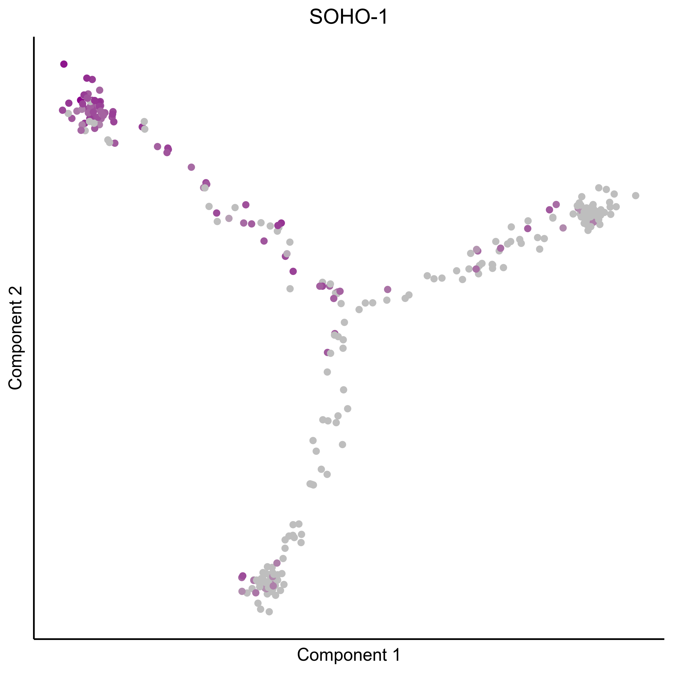
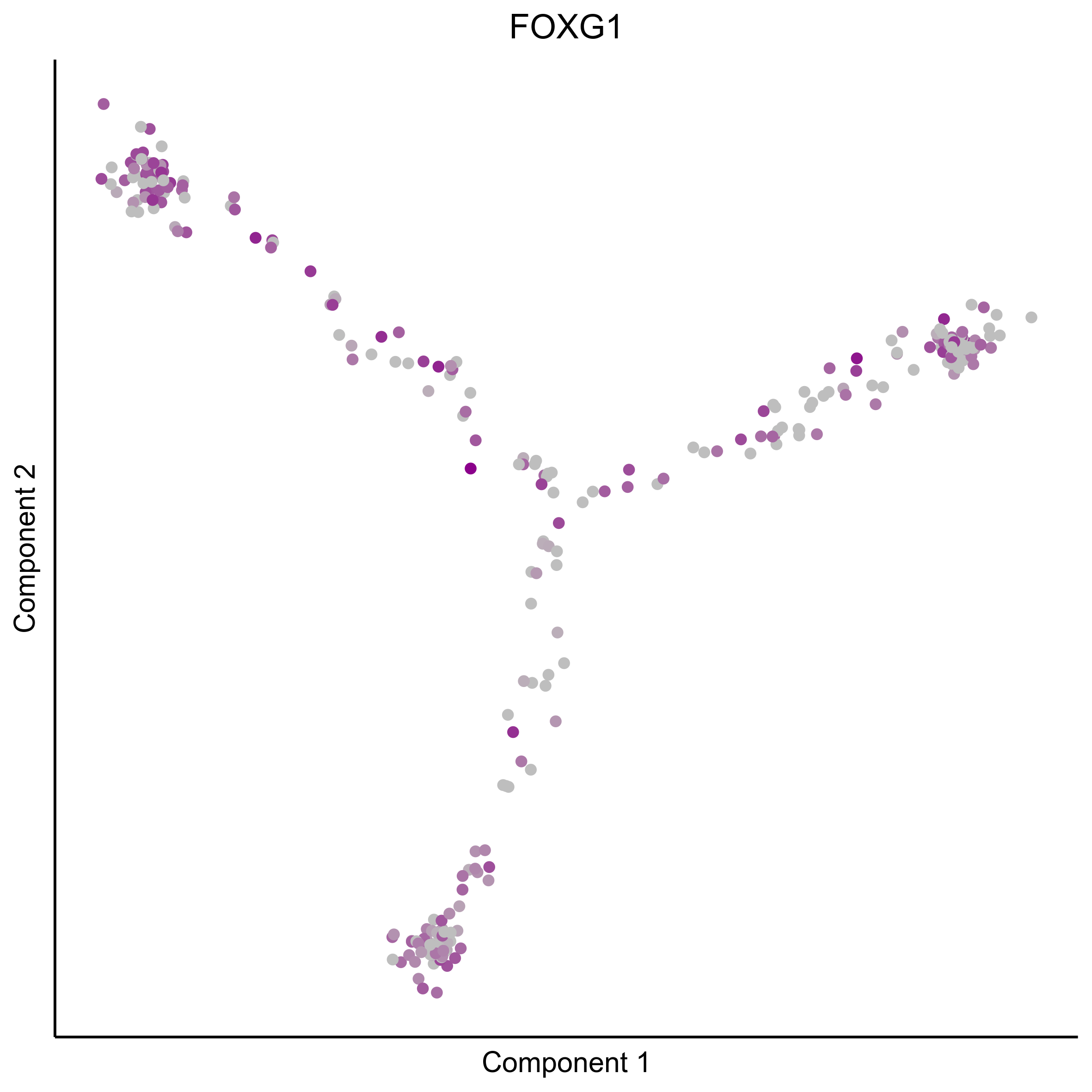
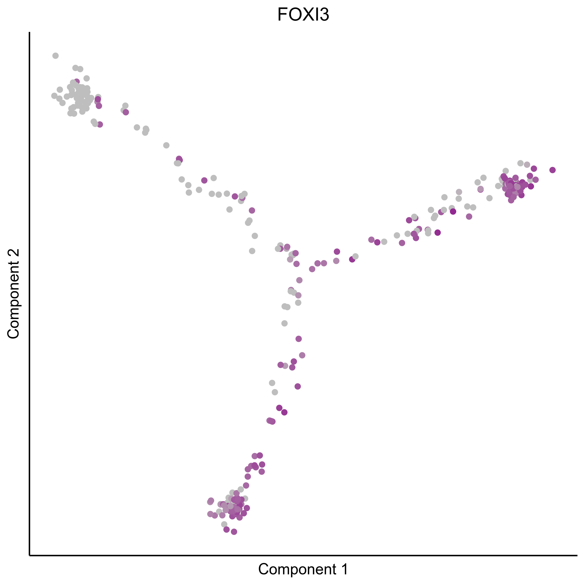
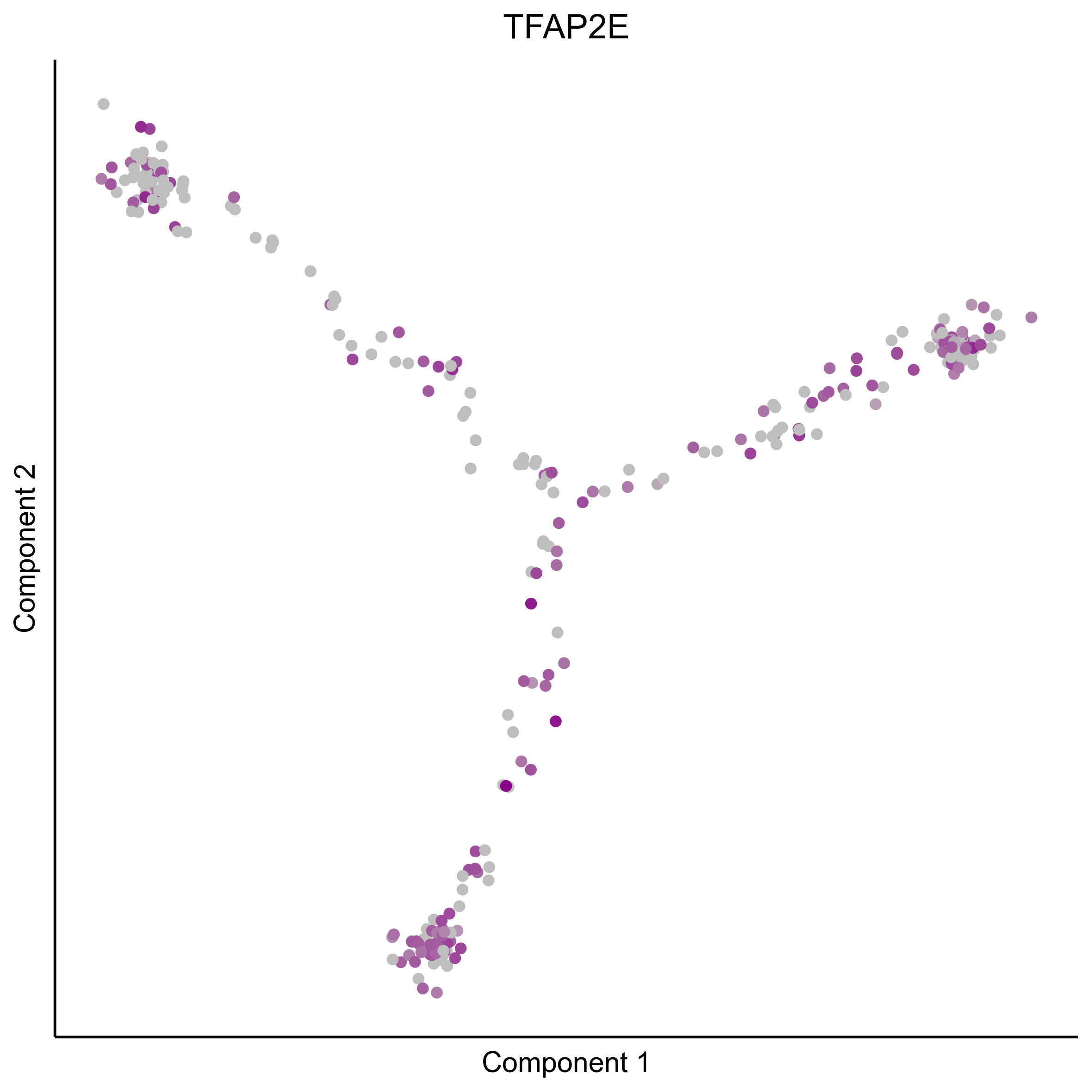
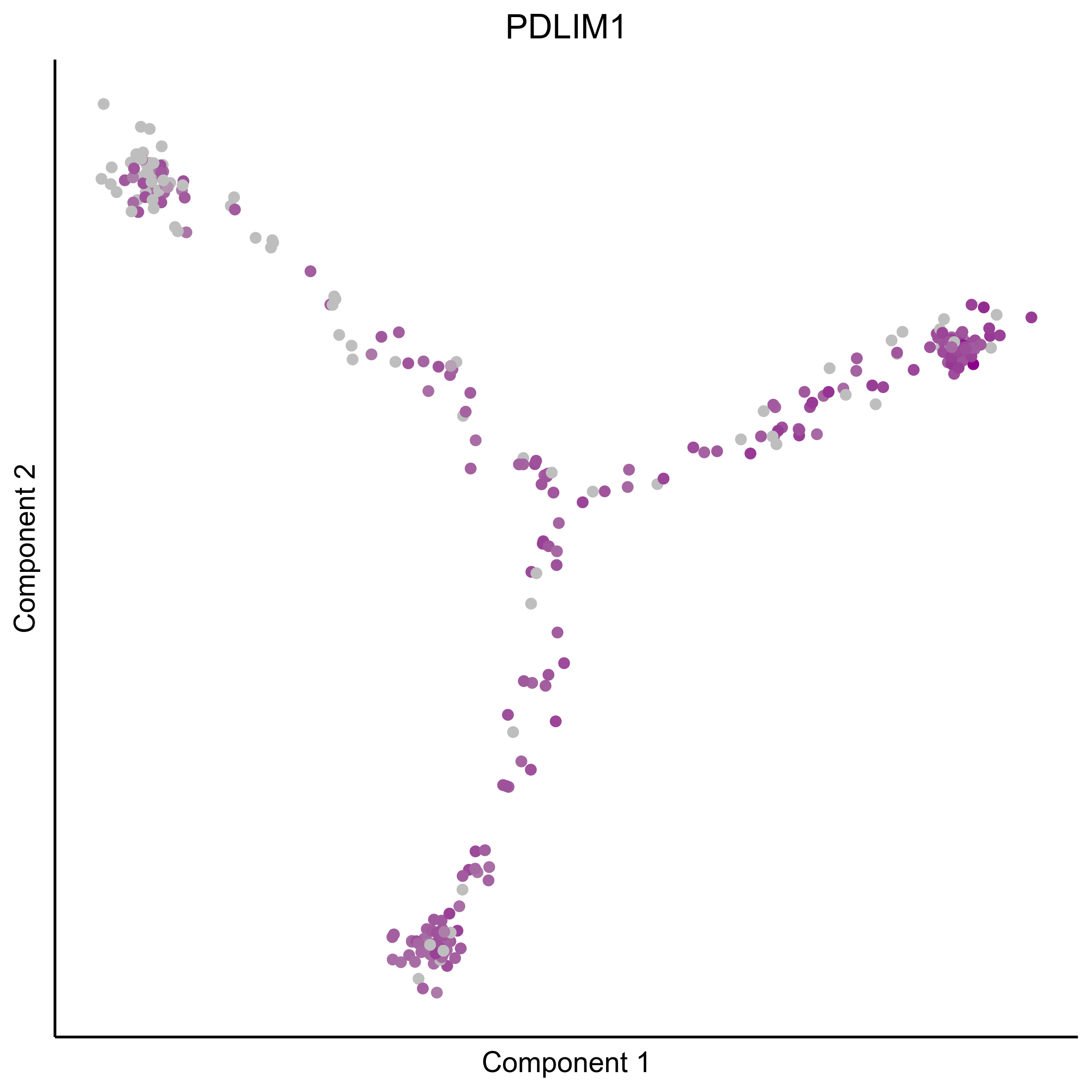
Plot gradient gene expression on Monocle embeddings.
curr_plot_folder = paste0(plot_path, "monocle_plots/gradient_plots/")
dir.create(curr_plot_folder)

for(gn in gene_list){
  png(paste0(curr_plot_folder, "monocle_gradient_", gn, '.png'), height = 15, width = 15, family = 'Arial', units = "cm", res = 400)
  print(ggplot(data.frame('Component 1' = reducedDimS(HSMM)[1,], 'Component 2' = reducedDimS(HSMM)[2,],
                          'colour_by' = as.integer(1+100*log10(1+m_oep$getReadcounts(data_status='Normalized')[gn,]) / max(log10(1+m_oep$getReadcounts(data_status='Normalized')[gn,]))),
                          check.names = FALSE),
               aes(x=`Component 1`, y=`Component 2`, color=colour_by)) +
          geom_point() +
          scale_color_gradient(low = "grey", high = "darkmagenta") +
          theme_classic() +
          theme(legend.position = "none", axis.ticks=element_blank(), axis.text = element_blank()) +
          ggtitle(gn) +
          theme(plot.title = element_text(hjust = 0.5)))
  graphics.off()
}
Download all Monocle gradient plots
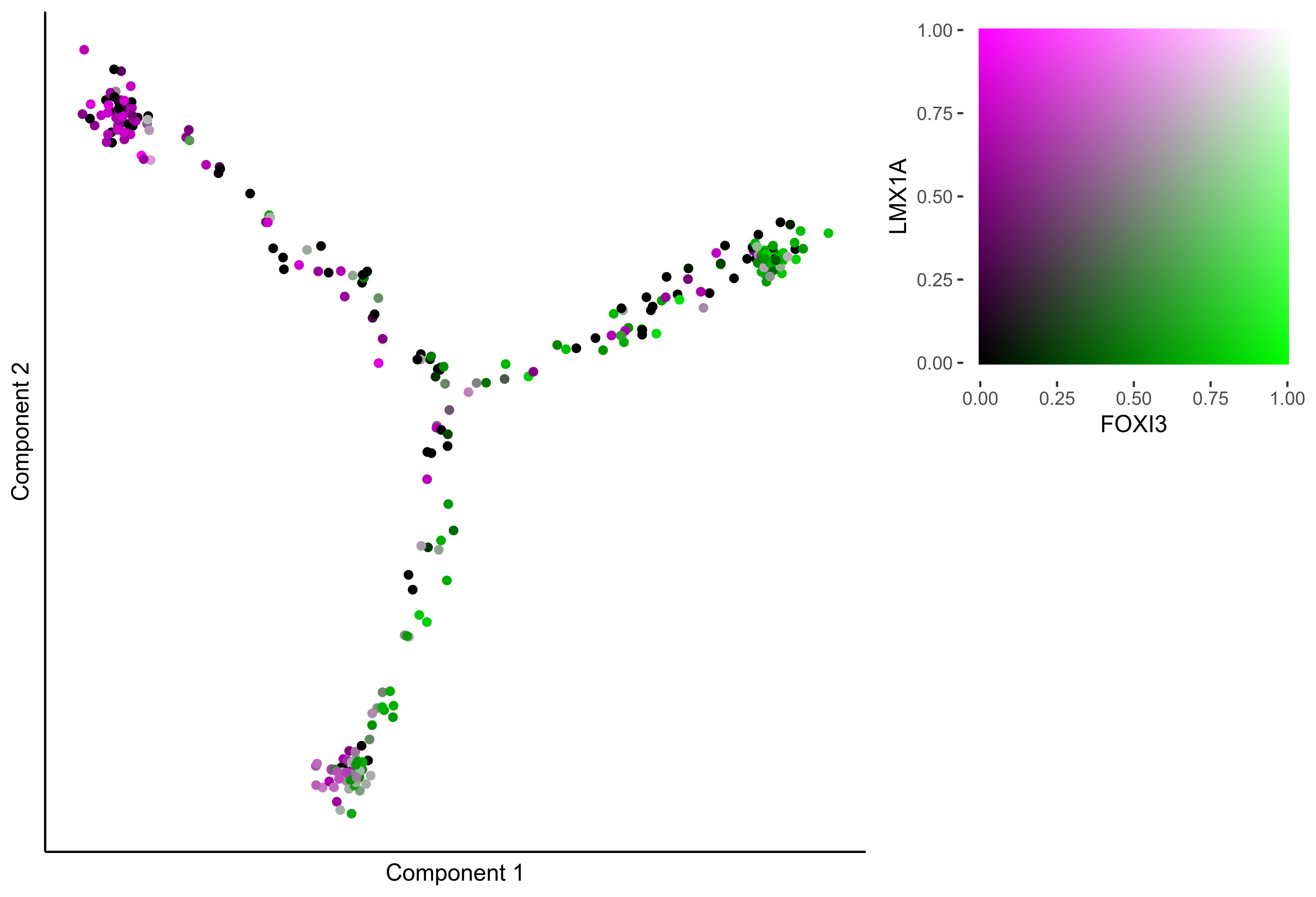
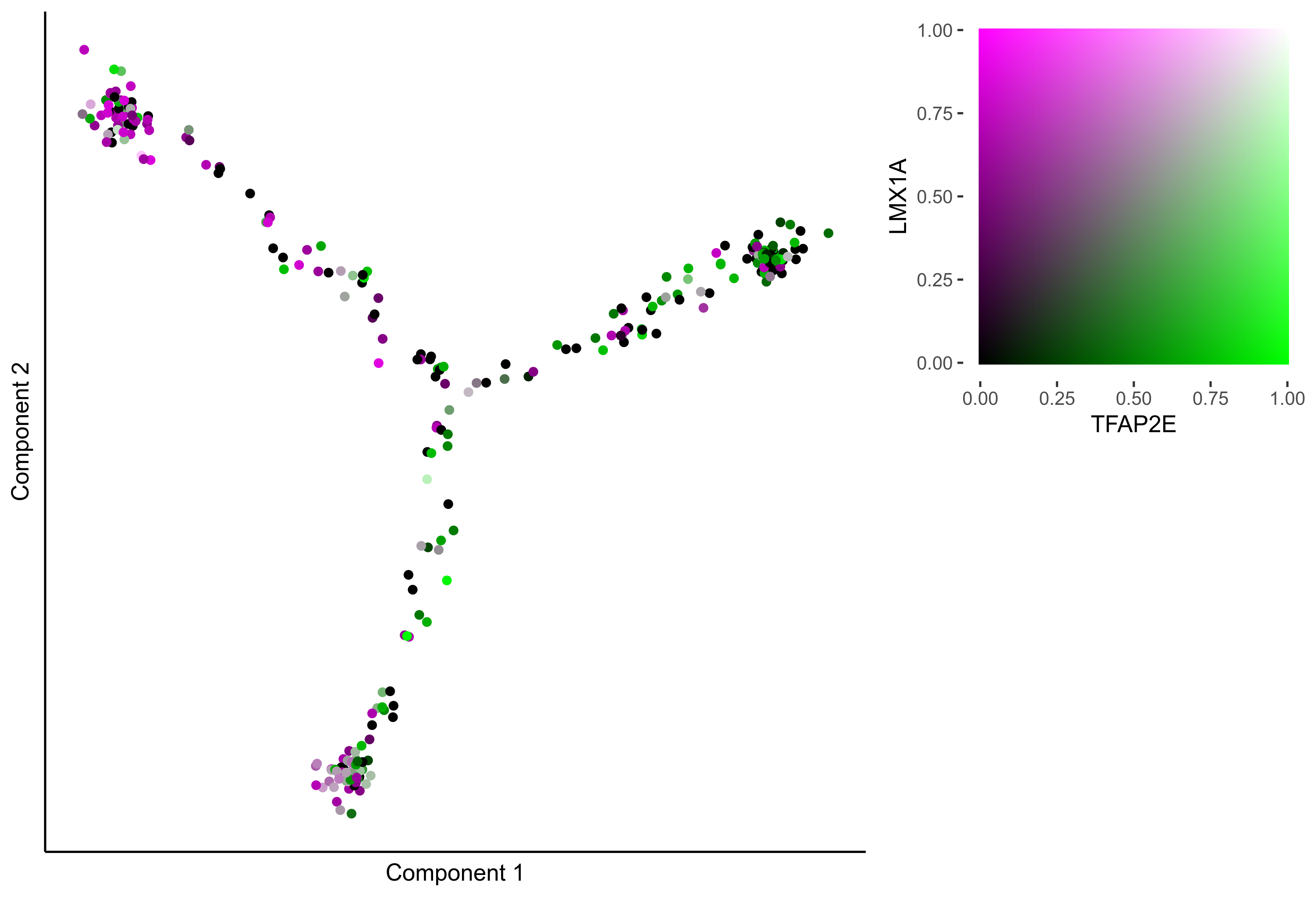
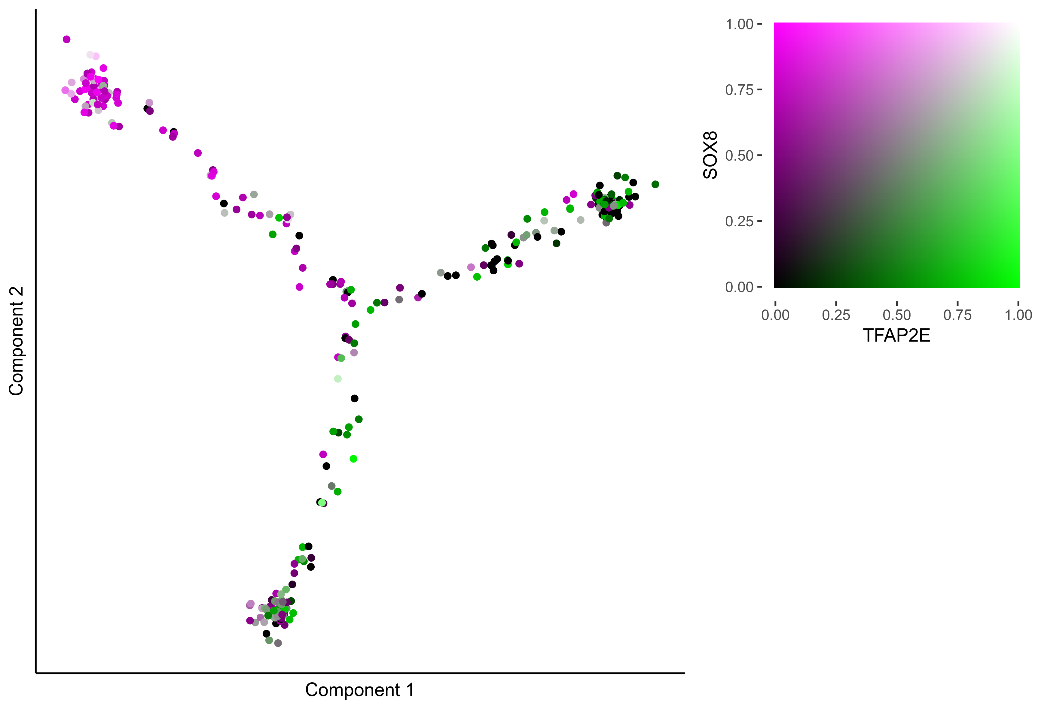
Plot Monocle co-expression plots.
curr_plot_folder = paste0(plot_path, "monocle_plots/coexpression/")
dir.create(curr_plot_folder)

# plot gradient gene co-expression on monocle embeddings
gene_pairs <- list(c("FOXI3", "LMX1A"), c("TFAP2E", "LMX1A"), c("FOXI3", "SOX8"), c("TFAP2E", "SOX8"))
lapply(gene_pairs, function(x) {monocle_coexpression_plot(m_oep, m_oep$topCorr_DR$genemodules.selected, monocle_obj = HSMM, gene1 = x[1], gene2 = x[2],
                                                          plot_folder = curr_plot_folder, height = 15, width = 22, res = 400, units = 'cm', family = 'Arial')})

Plot trajectories.
curr_plot_folder = paste0(plot_path, "monocle_plots/")
p1 = plot_cell_trajectory(HSMM, color_by = "cells_samples") +
scale_color_manual(values = c('#BBBDC1', '#6B98E9', '#05080D'), name = "cluster")
p2 = plot_cell_trajectory(HSMM, color_by = "Pseudotime") +
scale_color_gradient(low = "#008ABF", high = "#E53F00")
# Plot cell pseudotime
png(paste0(curr_plot_folder, 'Monocle_DDRTree_trajectories.png'), width=20, height=12, family = 'Arial', units = "cm", res = 400)
gridExtra::grid.arrange(grobs=list(p1, p2), layout_matrix=matrix(seq(2), ncol=2, byrow=T))
graphics.off()
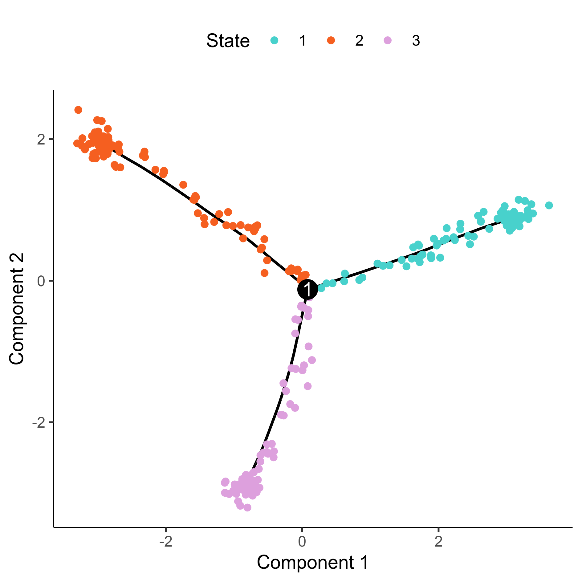
# Plot cell state
png(paste0(curr_plot_folder, 'Monocle_DDRTree_State_facet.png'), width=12, height=12, family = 'Arial', units = "cm", res = 400)
plot_cell_trajectory(HSMM, color_by = "State") +
scale_color_manual(values = c( '#48d1cc', '#f55f20', '#dda0dd'), name = "State")
graphics.off()
Generate a Monocle projection plot for each known gene.
curr_plot_folder = paste0(plot_path, "monocle_plots/all_monocle_projections/")
dir.create(curr_plot_folder)

genes_sel = sort(intersect(
  getDispersedGenes(m_oep$getReadcounts('Normalized'), -1),
  getHighGenes(m_oep$getReadcounts('Normalized'), mean_threshold=5)
))

gene_level = m_oep$getReadcounts("Normalized")[genes_sel %>% .[. %in% m_oep$getGeneNames()],]
gene_level.2 = t(apply(log(.1+gene_level), 1, function(x){
  pc_95 = quantile(x, .95)
  if(pc_95==0){
    pc_95=1
  }
  x <- x/pc_95
  x[x>1] <- 1
  as.integer(cut(x, breaks=10))
}))

for(n in rownames(gene_level.2)){
  print(n)
  pdf(paste0(curr_plot_folder, 'Monocle_DDRTree_projection_', n, '.pdf'))
  plot(t(reducedDimS(HSMM)), pch=16, main=n, xlab="", ylab="", xaxt='n', yaxt='n', asp=1,
       col=colorRampPalette(c("#0464DF", "#FFE800"))(n = 10)[gene_level.2[n,]]
  )
  graphics.off()
}

system(paste0("zip -rj ", plot_path, "monocle_plots/all_monocle_projections.zip ", curr_plot_folder))
unlink(curr_plot_folder, recursive=TRUE, force=TRUE)
Download Monocle plots for all known genes
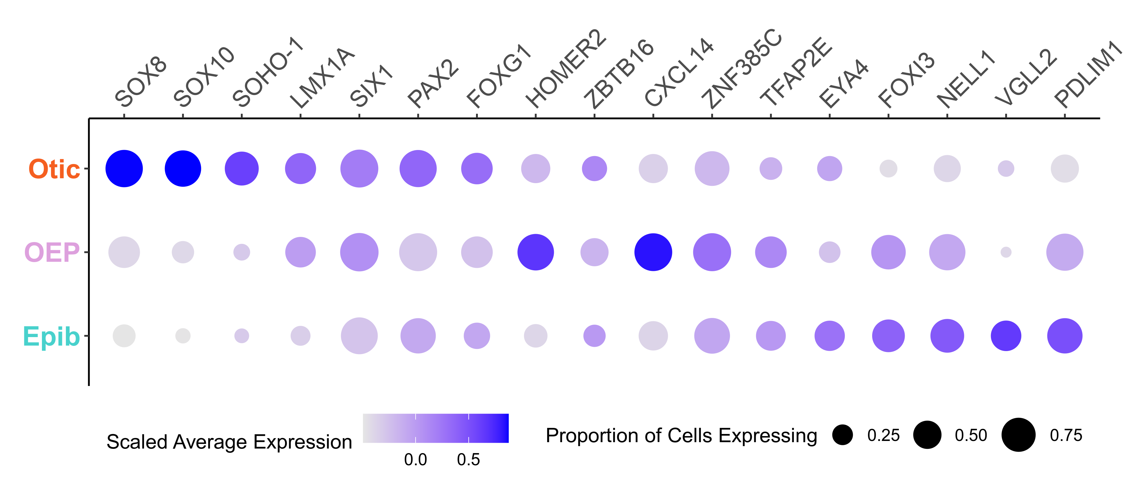
Plot dotplot for genes along Monocle branches.
curr_plot_folder = paste0(plot_path, "monocle_plots/")

# get cell branch information for dotplot
cell_branch_data = pData(HSMM)[, "State", drop=F] %>%
  tibble::rownames_to_column('cellname') %>%
  dplyr::rename(branch = State) %>%
  dplyr::mutate(celltype = case_when(
    branch == "1" ~ "Epib",
    branch == "2" ~ "Otic",
    branch == "3" ~ 'OEP'
  ))

# gather data for dotplot
dotplot_data <- data.frame(t(m_oep$getReadcounts('Normalized')[gene_list, ]), check.names=F) %>%
  tibble::rownames_to_column('cellname') %>%
  tidyr::gather(genename, value, -cellname) %>%
  dplyr::left_join(cell_branch_data, by="cellname") %>%
  dplyr::group_by(genename, celltype) %>%
  # calculate percentage of cells in each cluster expressing gene
  dplyr::mutate('Proportion of Cells Expressing' = sum(value > 0)/n()) %>%
  # scale data
  dplyr::group_by(genename) %>%
  dplyr::mutate(value = scale(value)) %>%
  # calculate mean expression
  dplyr::group_by(genename, celltype) %>%
  dplyr::mutate('Scaled Average Expression' = mean(value)) %>%
  dplyr::distinct(genename, celltype, .keep_all=TRUE) %>%
  dplyr::ungroup()

# order genes for dotplot based on divergent expression in otic and NC lineages
gene_order <- dotplot_data %>%
  select(genename, celltype, `Scaled Average Expression`) %>%
  filter(celltype %in% c('Otic', 'Epib')) %>%
  tidyr::pivot_wider(names_from = celltype,
              values_from = `Scaled Average Expression`) %>%
  dplyr::mutate(order = Otic-Epib) %>%
  arrange(-order) %>%
  dplyr::pull(genename)


# add gene order to dotplot_data
dotplot_data <- dotplot_data %>%
  dplyr::mutate(genename = factor(genename, levels = gene_order))

png(paste0(curr_plot_folder, "m_oep_dotplot.png"), width=24, height=10, family = 'Arial', units = "cm", res = 400)
ggplot(dotplot_data, aes(x=genename, y=celltype, size=`Proportion of Cells Expressing`, color=`Scaled Average Expression`)) +
  geom_count() +
  scale_size_area(max_size=10) +
  scale_x_discrete(position = "top") + xlab("") + ylab("") +
  scale_color_gradient(low = "grey90", high = "blue") +
  theme_classic() +
  theme(axis.text.x = element_text(angle = 45, hjust = 0, size=14),
        axis.text.y = element_text(colour =  c("#48d1cc", "#dda0dd", "#f55f20"), face = 'bold', size = 16),
        legend.position="bottom", legend.box = "horizontal", plot.margin=unit(c(0,1,0,0),"cm"), legend.text=element_text(size=10), legend.title=element_text(size=12))
graphics.off()
Plotting the expression of candidate genes, we can easliy classify the Otic, Epibranchial and OEP branches.
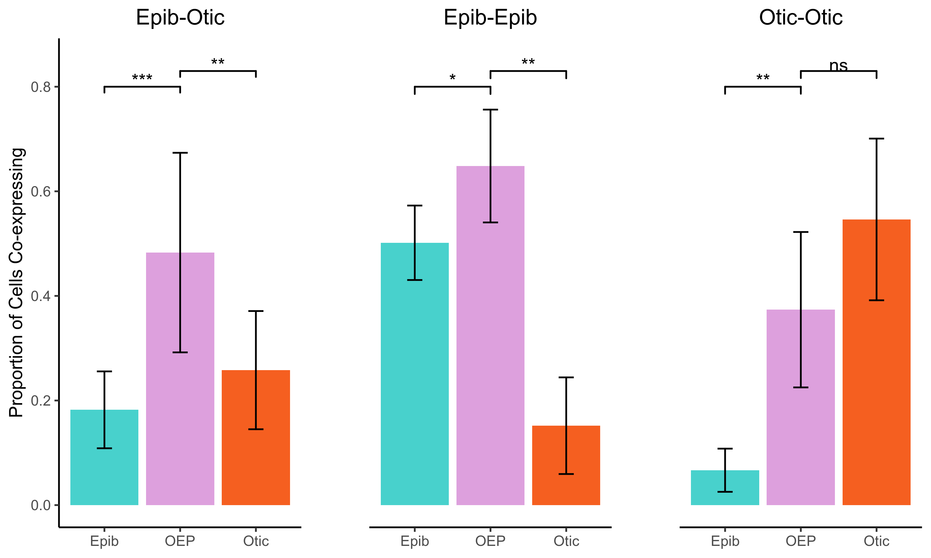
We calculate the co-expression of key Otic and Epibranchial markers along each of the Monocle branches. We then test and find that the level of co-expression of Otic and Epibranchial markers is higher in the OEP population relative to Otic and Epibranchial branches. This shows that individual OEP cells are co-expressing markers of both lineages - indicative of a bipotent progenenitor population.
First we determine the list of genes used for co-expression analysis.
otic = c("SOX10", "SOX8", "HOMER2", 'LMX1A')
epi = c("NELL1", "FOXI3", "PDLIM1", "TFAP2E")
For each gene pair we calculate the proportion of cells which express both genes in each Monocle branch.
# generate gene pairs for coexpression
comb <- t(combn(c(otic, epi), 2))

# use data cell branch data from dotplots
coexpression_data = data.frame()
for(pair in 1:nrow(comb)){
  if(sum(as.character(comb[pair,]) %in% otic) == 2){comparison = "o-o"}else if(sum(as.character(comb[pair,]) %in% otic) == 1){comparison = "o-e"}else{comparison = "e-e"}
  newdat = ldply(unique(cell_branch_data$celltype), function(y) {
    c(sum(colSums(m_oep$getReadcounts(data_status='Normalized')[c(comb[pair,1], comb[pair,2]), cell_branch_data[cell_branch_data$celltype == y, 'cellname']] > 0) == 2)/sum(cell_branch_data$celltype == y),
      comparison, y)
  })
  newdat[,1] <- as.numeric(newdat[,1])
  coexpression_data = rbind(coexpression_data, newdat)
}

# rename dataframe columns
colnames(coexpression_data) = c("value", "comparison", "branch")
We then carry out a non-parametric Kruskal Wallis test to compare the proportions of cells co-expressing pairs of genes across Monocle branches. Pairwise comparisons, comparing Otic and Epibranchial lineages to the control OEP lineage, were carried out using Wilcoxon rank sum tests.
# test co-expression in OEP lineage and epibranchial/otic branches
coexpression_stats <- coexpression_data %>%
  mutate(branch = factor(branch, levels = c("OEP", "Epib", "Otic"))) %>%
  group_split(comparison)

names(coexpression_stats) <- lapply(coexpression_stats, function(x) as.character(unique(x[["comparison"]])))

# Non parametric kruskal wallis test
lapply(coexpression_stats, function(x) kruskal.test(value ~ branch, data = x))

# Wilcoxon rank sum test
lapply(coexpression_stats, function(x) filter(x, branch == 'OEP' | branch == "Otic") %>% wilcox.test(value ~ branch, data = .))
lapply(coexpression_stats, function(x) filter(x, branch == 'OEP' | branch == "Epib") %>% wilcox.test(value ~ branch, data = .))
We calculate the average proportion of cells co-expressing pairs of genes and plot the output.
# calculate mean value per group and SD for plotting bar plot
plot_dat <- coexpression_data %>%
  dplyr::group_by(branch, comparison) %>%
  dplyr::summarise(
    "Proportion of Cells Co-expressing" = mean(value, na.rm = TRUE),
    sd = sd(value, na.rm = TRUE)
  ) %>%
  dplyr::ungroup() %>%
  group_split(comparison)

# rename dataframes split by comparison
names(plot_dat) <- lapply(plot_dat, function(x) as.character(unique(x[["comparison"]])))

# bar plots
oe_plot <- ggplot(plot_dat$`o-e`, aes(x=branch,y=`Proportion of Cells Co-expressing`, fill = branch)) +
  geom_bar(stat='identity') +
  scale_fill_manual("legend", values = c("Otic" = "#f55f20", "Epib" = "#48d1cc", "OEP" = "#dda0dd")) +
  geom_errorbar(aes(ymin=`Proportion of Cells Co-expressing`-sd, ymax=`Proportion of Cells Co-expressing`+sd), width=.2,
                position=position_dodge(.9)) +
  geom_signif(comparisons=list(c("OEP", "Otic")), annotations = "**",
              y_position = 0.83, tip_length = 0.02, vjust=0.4) +
  geom_signif(comparisons=list(c("OEP", "Epib")), annotations = "***",
              y_position = 0.8, tip_length = 0.02, vjust=0.4) +
  ylim(c(0, 0.85)) +
  theme_classic() +
  theme(axis.title.x=element_blank(),
        legend.position="none") +
  ggtitle("Epib-Otic") +
  theme(plot.title = element_text(hjust = 0.5))

ee_plot <- ggplot(plot_dat$`e-e`, aes(x=branch,y=`Proportion of Cells Co-expressing`, fill = branch)) +
  geom_bar(stat='identity') +
  scale_fill_manual("legend", values = c("Otic" = "#f55f20", "Epib" = "#48d1cc", "OEP" = "#dda0dd")) +
  geom_errorbar(aes(ymin=`Proportion of Cells Co-expressing`-sd, ymax=`Proportion of Cells Co-expressing`+sd), width=.2,
                position=position_dodge(.9)) +
  geom_signif(comparisons=list(c("OEP", "Otic")), annotations = "**",
              y_position = 0.83, tip_length = 0.02, vjust=0.4) +
  geom_signif(comparisons=list(c("OEP", "Epib")), annotations = "*",
              y_position = 0.8, tip_length = 0.02, vjust=0.4) +
  ylim(c(0, 0.85)) +
  theme_classic() +
  theme(axis.title.y =element_blank(),
        axis.text.y=element_blank(),
        axis.ticks.y=element_blank(),
        axis.line.y = element_blank(),
        axis.title.x=element_blank(),
        legend.position="none") +
  ggtitle("Epib-Epib") +
  theme(plot.title = element_text(hjust = 0.5))


oo_plot <- ggplot(plot_dat$`o-o`, aes(x=branch,y=`Proportion of Cells Co-expressing`, fill = branch)) +
  geom_bar(stat='identity') +
  scale_fill_manual("legend", values = c("Otic" = "#f55f20", "Epib" = "#48d1cc", "OEP" = "#dda0dd")) +
  geom_errorbar(aes(ymin=`Proportion of Cells Co-expressing`-sd, ymax=`Proportion of Cells Co-expressing`+sd), width=.2,
                position=position_dodge(.9)) +
  geom_signif(comparisons=list(c("OEP", "Otic")), annotations = "ns",
              y_position = 0.83, tip_length = 0.02, vjust=0.4) +
  geom_signif(comparisons=list(c("OEP", "Epib")), annotations = "**",
              y_position = 0.8, tip_length = 0.02, vjust=0.4) +
  ylim(c(0, 0.85)) +
  theme_classic() +
  theme(axis.title.y=element_blank(),
        axis.text.y=element_blank(),
        axis.ticks.y=element_blank(),
        axis.line.y=element_blank(),
        axis.title.x=element_blank(),
        legend.position="none") +
  ggtitle("Otic-Otic") +
  theme(plot.title = element_text(hjust = 0.5))

png(paste0(curr_plot_folder, "coexpression_test.png"), width=20, height=12, family = 'Arial', units = "cm", res = 400)
plot_grid(oe_plot, ee_plot, oo_plot, align = "hv", nrow = 1, rel_widths = c(1,1,1))
graphics.off()
From these three plots we can see that the co-expression of Epibranchial and Otic genes is significantly higher in the OEP branch relative to Otic and Epibranchial branches. This is not the case with the co-expression of pairs of Otic genes or pairs of Epibranchial genes.
BEAM is used to identify genes with branch dependent expression.
We select genes with high expression and dispersion, and then use BEAM QC to filter and plot their expression across pseudotime.
genes_sel = intersect(
  getDispersedGenes(m_oep$getReadcounts('Normalized'), -1),
  getHighGenes(m_oep$getReadcounts('Normalized'), mean_threshold=5)
)

branch_point_id = 1
BEAM_res <- BEAM(HSMM[genes_sel, ], branch_point = branch_point_id, cores = m_oep$num_cores)

BEAM_res <- BEAM_res[order(BEAM_res$qval),]
BEAM_res <- BEAM_res[,c("gene_short_name", "pval", "qval")]

png(paste0(curr_plot_folder, 'Monocle_Beam.png'), width=20, height=100, family = 'Arial', units = "cm", res = 400)
beam_hm = plot_genes_branched_heatmap(HSMM[row.names(subset(BEAM_res, qval < .05)),],
                                      branch_point = branch_point_id,
                                      num_clusters = 20,
                                      cores = ncores,
                                      use_gene_short_name = T,
                                      show_rownames = T,
                                      return_heatmap=T,
                                      branch_colors=c('#dd70dd', '#48d1cc', '#f55f20'),
                                      branch_labels=c("Epib", 'Otic'))
graphics.off()

# save beam score to file
write.csv(BEAM_res %>% dplyr::arrange(pval), paste0(curr_plot_folder, 'beam_scores.csv'), row.names=F)
Plot BEAM for original favourite genes.
png(paste0(curr_plot_folder, 'Monocle_Beam_knownGenes.png'), width=20, height=25, family = 'Arial', units = "cm", res = 400)
beam_hm = plot_genes_branched_heatmap(HSMM[m_oep$favorite_genes,],
                                      branch_point = branch_point_id,
                                      cores = 1,
                                      use_gene_short_name = T,
                                      show_rownames = T,
                                      return_heatmap=T,
                                      branch_colors=c('#dd70dd', '#48d1cc', '#f55f20'),
                                      branch_labels=c("Epib", 'Otic'))
graphics.off()
Plot BEAM for selected markers.
beam_gene_list = c(gene_list, 'SOX13', 'TFAP2A', 'GATA3', 'EPHA4', 'DLX5', 'PRDM1', 'PRDM12', 'EYA1', 'EYA2', 'ETV4')

png(paste0(curr_plot_folder, 'Monocle_Beam_selGenes.png'), width=16, height=10, family = 'Arial', units = "cm", res = 400)
beam_hm = plot_genes_branched_heatmap(HSMM[beam_gene_list,],
                                      branch_point = branch_point_id,
                                      cluster_rows=FALSE,
                                      num_clusters = 4,
                                      cores = 1,
                                      use_gene_short_name = T,
                                      show_rownames = T,
                                      return_heatmap=T,
                                      branch_colors=c('#dd70dd', '#48d1cc', '#f55f20'),
                                      branch_labels=c("Epib", 'Otic'))
graphics.off()
RNA velocity uses the abundance of spliced and un-spliced RNA transcripts, in order to infer the future state of single cells.
First, we read in splice counts (Loom data) and filter cells and genes remaining in OEP subset.
curr_plot_folder = paste0(plot_path, "velocyto/")
dir.create(curr_plot_folder)

# read in loom data, with ensembl ID as rownames instead of gene name
velocyto_dat <- custom_read_loom(list.files(velocyto_input, pattern = '*.loom', full.names = T))

# change cell names in velocyto dat to match antler cell names
velocyto_dat <- lapply(velocyto_dat, function(x) {
  colnames(x) <- gsub(".*:", "", colnames(x))
  colnames(x) <- gsub("\\..*", "", colnames(x))
  colnames(x) <- unname(sapply(colnames(x), function(y) ifelse(
    grepl("ss8-TSS", y),
    sapply(strsplit(y, split = "_"), function(z){paste0(z[[2]], z[[3]])}),
    strsplit(y, split = "_")[[1]][[3]])))
  x
})

# get gene annotations from antler object
antler.gene.names <- m_oep$expressionSet@featureData@data

# keep only cells in m_oep
m_oep_velocyto_dat <- lapply(velocyto_dat,function(x) {
  x[,colnames(x) %in% names(m_oep$cellClusters$Mansel$cell_ids)]
})

# keep only genes in cleaned antler dataset and rename genes based on antler names
m_oep_velocyto_dat <- lapply(m_oep_velocyto_dat, function(x){
  x <- x[rownames(x) %in% fData(m_oep$expressionSet)$ensembl_gene_id,]
  rownames(x) <- fData(m_oep$expressionSet)$current_gene_names[match(rownames(x), fData(m_oep$expressionSet)$ensembl_gene_id)]
  x
})
Extract count matrices for spliced, un-spliced and spanning reads, and calculate RNA velocity.
# exonic read (spliced) expression matrix
emat <- m_oep_velocyto_dat$spliced
# intronic read (unspliced) expression matrix
nmat <- m_oep_velocyto_dat$unspliced
# spanning read (intron+exon) expression matrix
smat <- m_oep_velocyto_dat$spanning

# calculate cell velocity
rvel <- gene.relative.velocity.estimates(emat,nmat,smat=smat, kCells = 5, diagonal.quantiles = TRUE, fit.quantile = 0.05, n.cores = ncores)
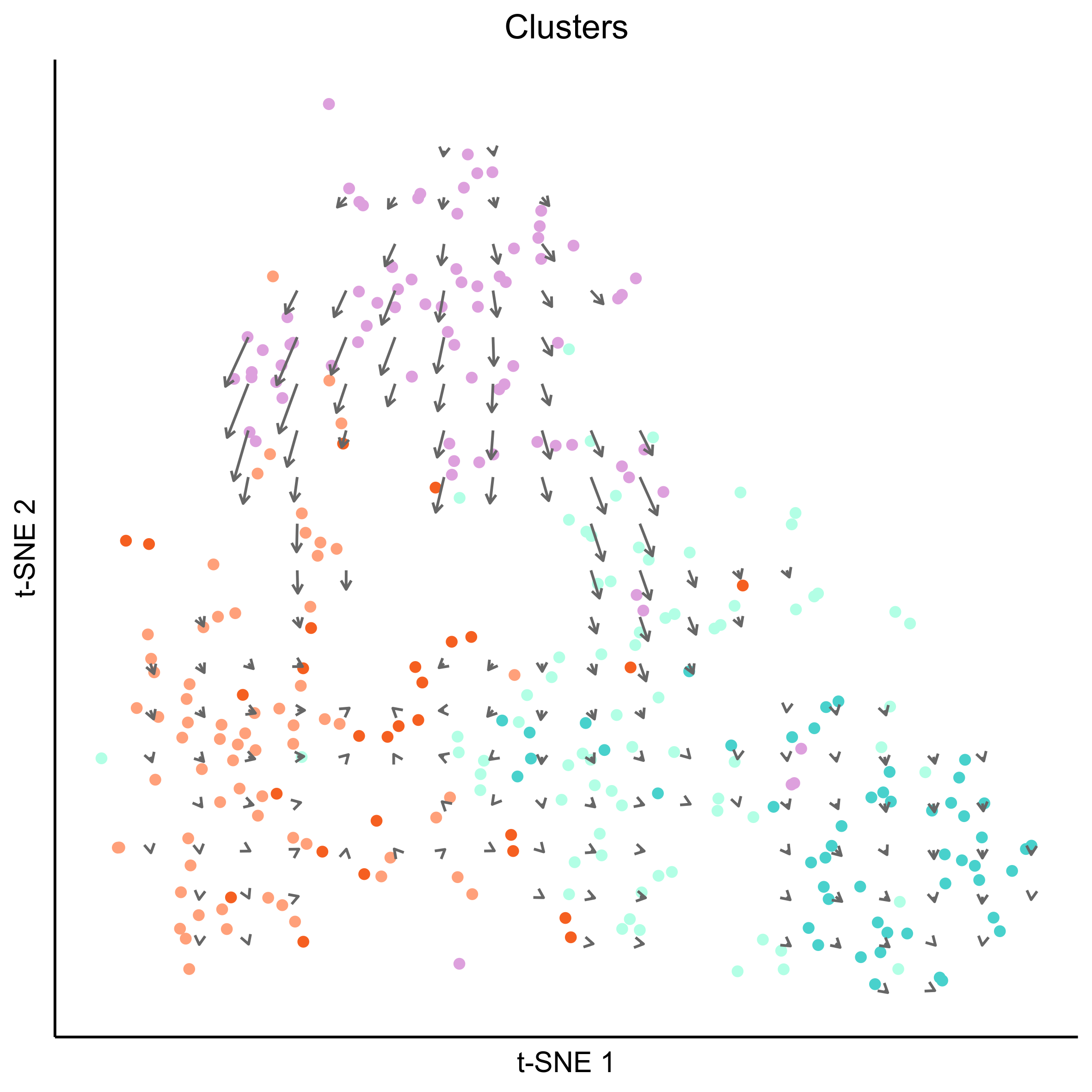
Plot RNA velocity on tSNE embeddings for cell clusters.
# get tsne embeddings for m_oep cells
tsne.embeddings = tsne_embeddings(m_oep, m_oep$topCorr_DR$genemodules.selected, seed=seed, perplexity=perp, pca=FALSE, eta=eta)

# return velocity object to plot with ggplot
vector_dat <- show.velocity.on.embedding.cor(tsne.embeddings, rvel, n=100, scale='sqrt',
                               cex=1.5, arrow.scale=8, arrow.lwd=1.5, n.cores = ncores,
                               show.grid.flow=TRUE, min.grid.cell.mass=0.5,grid.n=20, return.details = TRUE)

# plot vector map on clusters
png(paste0(curr_plot_folder, 'OEP_subset_velocity_clusters_vector.png'), height = 15, width = 15, family = 'Arial', units = "cm", res = 400)
tsne_plot(m_oep, m_oep$topCorr_DR$genemodules.selected, seed=seed, colour_by=m_oep$cellClusters[['Mansel']]$cell_ids, colours=clust.colors, perplexity=perp, eta=eta) +
  ggtitle('Clusters') +
  theme(plot.title = element_text(hjust = 0.5)) +
  geom_segment(data = as.data.frame(vector_dat$garrows),
               aes(x = x0, xend = x1, y = y0, yend = y1),
               size = 0.5,
               arrow = arrow(length = unit(4, "points"), type = "open"),
               colour = "grey40")
graphics.off()

# plot cell arrows on clusters
png(paste0(curr_plot_folder, 'OEP_subset_velocity_clusters_arrows.png'), height = 15, width = 15, family = 'Arial', units = "cm", res = 400)
tsne_plot(m_oep, m_oep$topCorr_DR$genemodules.selected, seed=seed, colour_by=m_oep$cellClusters[['Mansel']]$cell_ids, colours=clust.colors, perplexity=perp, eta=eta) +
  ggtitle('Clusters') +
  theme(plot.title = element_text(hjust = 0.5)) +
  geom_segment(data = as.data.frame(vector_dat$arrows),
               aes(x = x0, xend = x1, y = y0, yend = y1),
               size = 0.5,
               arrow = arrow(length = unit(4, "points"), type = "open"),
               colour = "grey40")
graphics.off()
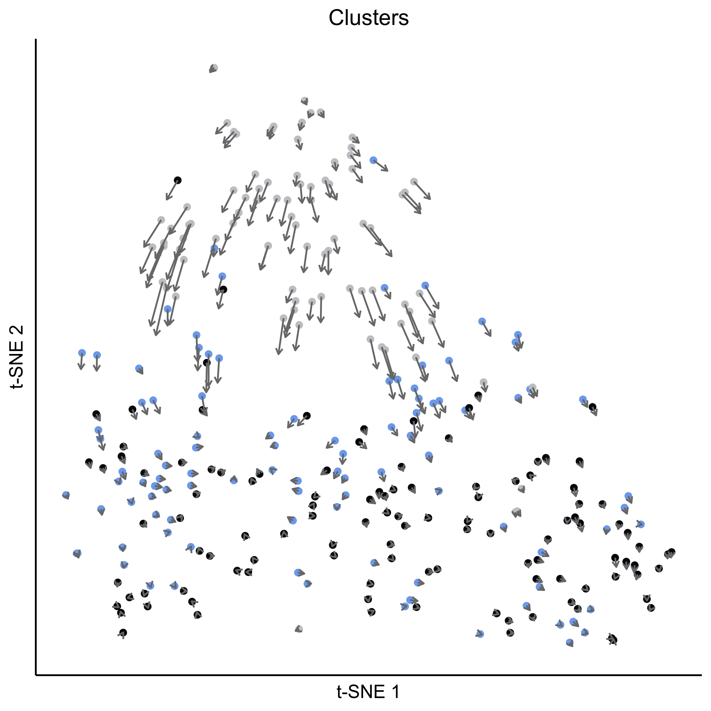
Plot RNA velocity on tSNE embeddings for developmental stage.
# plot vector map on stage
png(paste0(curr_plot_folder, 'OEP_subset_velocity_stage_vector.png'), height = 15, width = 15, family = 'Arial', units = "cm", res = 400)
tsne_plot(m_oep, m_oep$topCorr_DR$genemodules.selected, seed=seed, colour_by=pData(m_oep$expressionSet)$timepoint, colours = stage_cols, perplexity=perp, eta=eta) +
ggtitle('Clusters') +
theme(plot.title = element_text(hjust = 0.5)) +
geom_segment(data = as.data.frame(vector_dat$garrows),
aes(x = x0, xend = x1, y = y0, yend = y1),
size = 0.5,
arrow = arrow(length = unit(4, "points"), type = "open"),
colour = "grey40")
graphics.off()
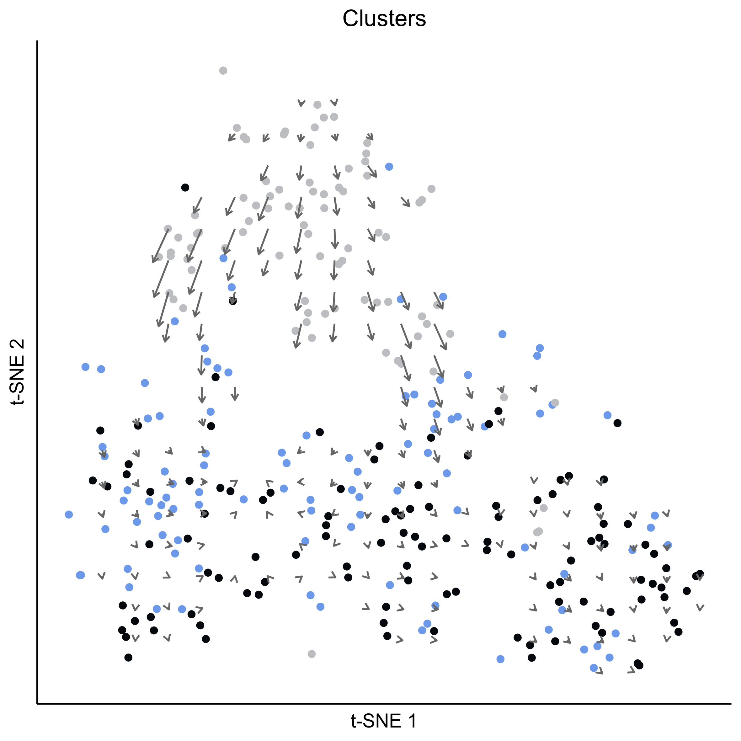
# plot cell arrows on stage
png(paste0(curr_plot_folder, 'OEP_subset_velocity_stage_arrows.png'), height = 15, width = 15, family = 'Arial', units = "cm", res = 400)
tsne_plot(m_oep, m_oep$topCorr_DR$genemodules.selected, seed=seed, colour_by=pData(m_oep$expressionSet)$timepoint, colours = stage_cols, perplexity=perp, eta=eta) +
ggtitle('Clusters') +
theme(plot.title = element_text(hjust = 0.5)) +
geom_segment(data = as.data.frame(vector_dat$arrows),
aes(x = x0, xend = x1, y = y0, yend = y1),
size = 0.5,
arrow = arrow(length = unit(4, "points"), type = "open"),
colour = "grey40")
graphics.off()
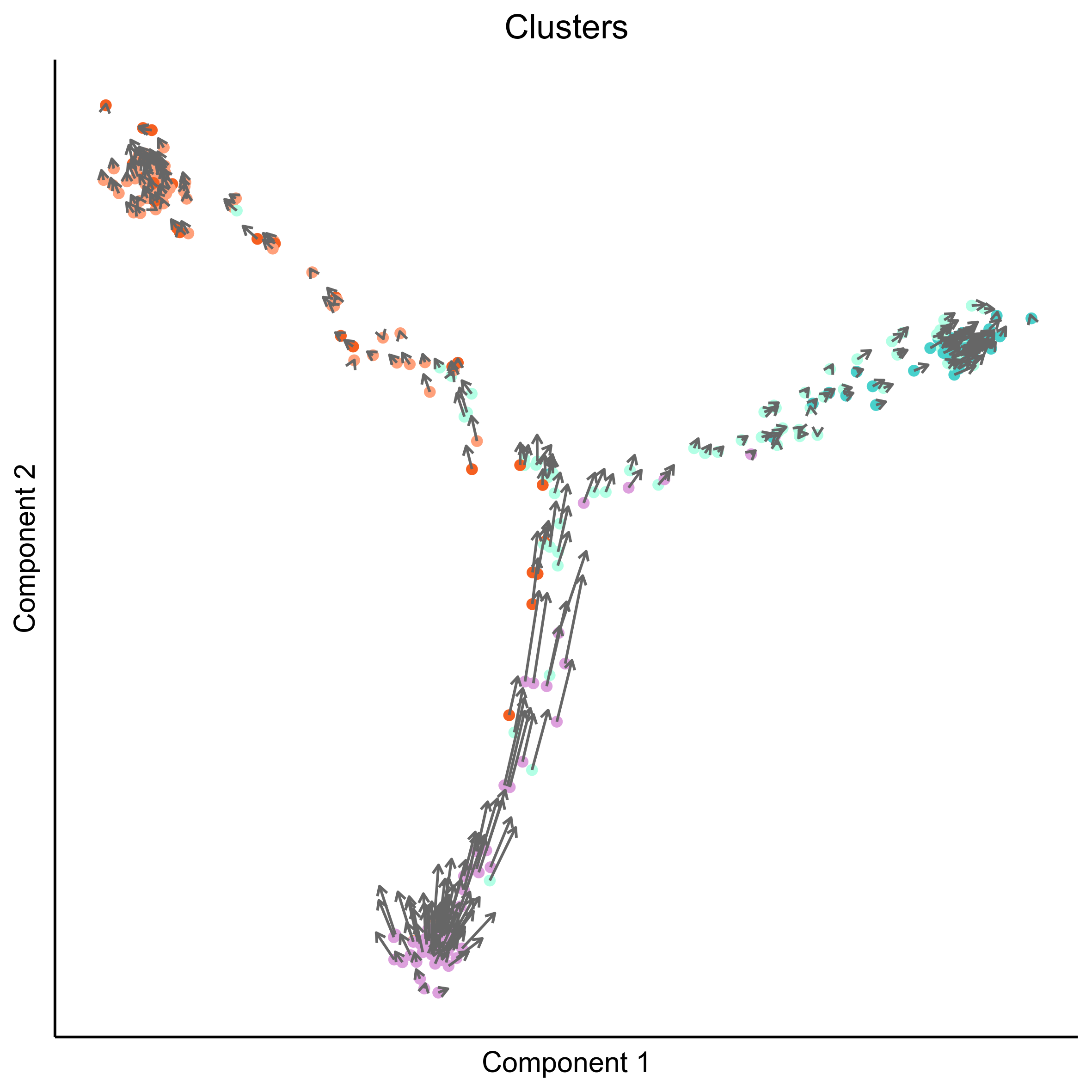
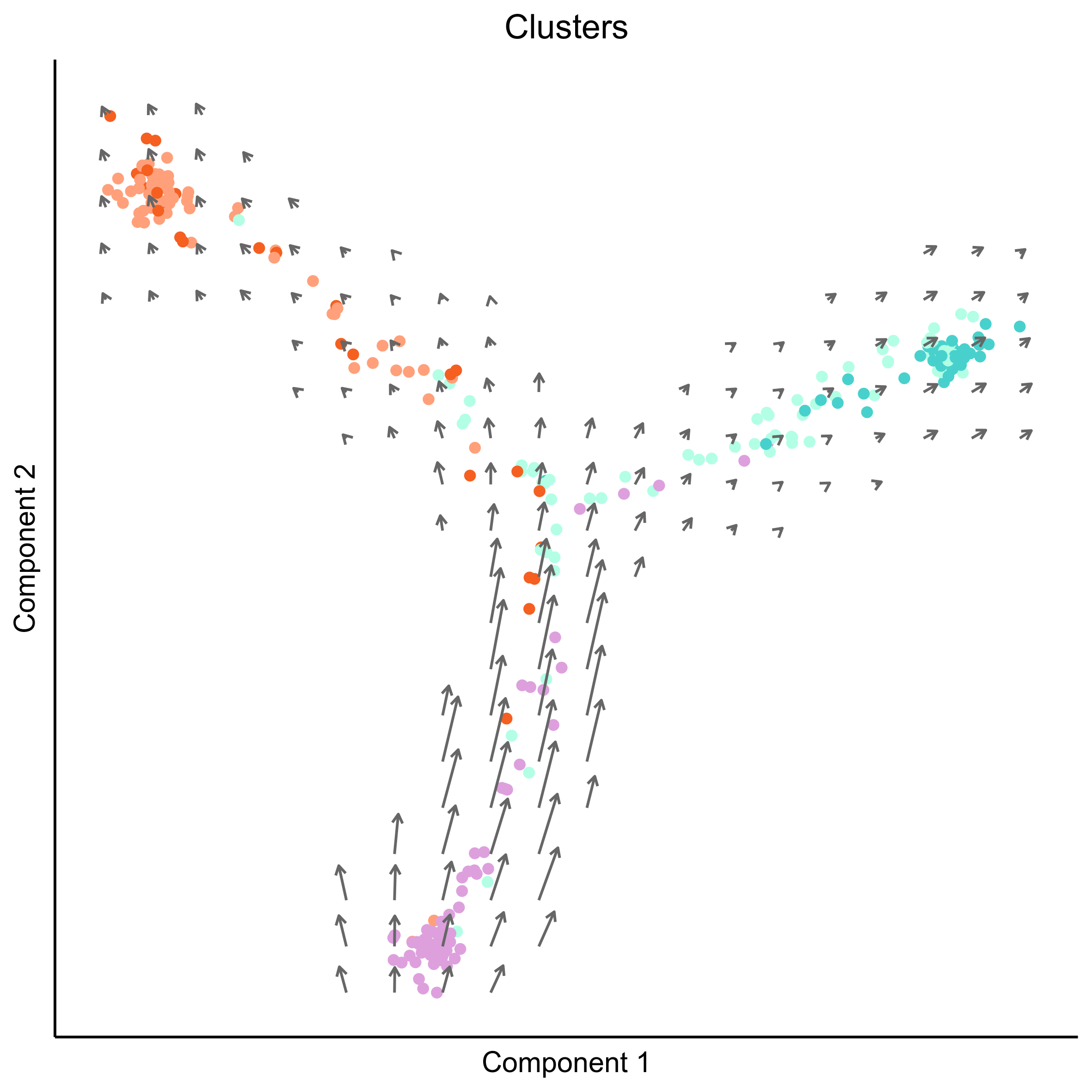
Plot RNA velocity on Monocle embeddings for cell clusters.
# return velocity object to plot with ggplot
vector_dat <- show.velocity.on.embedding.cor(t(reducedDimS(HSMM)), rvel, n=100, scale='sqrt',
                                             cex=1.5, arrow.scale=1, arrow.lwd=1.2, cell.border.alpha = 0, n.cores = ncores,
                                             show.grid.flow=TRUE, min.grid.cell.mass=0.5,grid.n=20, return.details = TRUE)
graphics.off()

# plot vector map on clusters
png(paste0(curr_plot_folder, 'Monocle_velocity_clusters_vector.png'), height = 15, width = 15, family = 'Arial', units = "cm", res = 400)
ggplot(data.frame('Component 1' = reducedDimS(HSMM)[1,], 'Component 2' = reducedDimS(HSMM)[2,],
                  'colour_by' = as.factor(m_oep$cellClusters[['Mansel']]$cell_ids), check.names = FALSE), aes(x=`Component 1`, y=`Component 2`, color=colour_by)) +
  geom_point() +
  scale_color_manual(values = clust.colors) +
  geom_segment(data = as.data.frame(vector_dat$garrows),
               aes(x = x0, xend = x1, y = y0, yend = y1),
               size = 0.5,
               arrow = arrow(length = unit(4, "points"), type = "open"),
               colour = "grey40") +
  theme_classic() +
  theme(legend.position = "none", axis.ticks=element_blank(), axis.text = element_blank()) +
  ggtitle('Clusters') +
  theme(plot.title = element_text(hjust = 0.5))
graphics.off()

# plot cell arrows on clusters
png(paste0(curr_plot_folder, 'Monocle_velocity_clusters_arrows.png'), height = 15, width = 15, family = 'Arial', units = "cm", res = 400)
ggplot(data.frame('Component 1' = reducedDimS(HSMM)[1,], 'Component 2' = reducedDimS(HSMM)[2,],
                  'colour_by' = as.factor(m_oep$cellClusters[['Mansel']]$cell_ids), check.names = FALSE), aes(x=`Component 1`, y=`Component 2`, color=colour_by)) +
  geom_point() +
  scale_color_manual(values = clust.colors) +
  geom_segment(data = as.data.frame(vector_dat$arrows),
               aes(x = x0, xend = x1, y = y0, yend = y1),
               size = 0.5,
               arrow = arrow(length = unit(4, "points"), type = "open"),
               colour = "grey40") +
  theme_classic() +
  theme(legend.position = "none", axis.ticks=element_blank(), axis.text = element_blank()) +
  ggtitle('Clusters') +
  theme(plot.title = element_text(hjust = 0.5))
graphics.off()
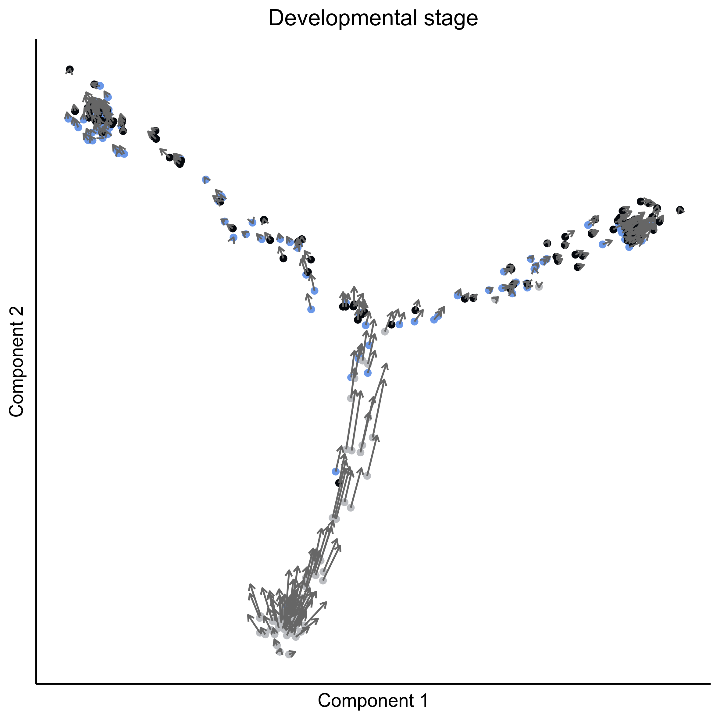
Plot RNA velocity on Monocle embeddings for developmental stage.
# plot vector map on stage
png(paste0(curr_plot_folder, 'Monocle_velocity_stage_vector.png'), height = 15, width = 15, family = 'Arial', units = "cm", res = 400)
ggplot(data.frame('Component 1' = reducedDimS(HSMM)[1,], 'Component 2' = reducedDimS(HSMM)[2,],
'colour_by' = as.factor(pData(m_oep$expressionSet)$timepoint), check.names = FALSE), aes(x=`Component 1`, y=`Component 2`, color=colour_by)) +
geom_point() +
scale_color_manual(values = stage_cols) +
geom_segment(data = as.data.frame(vector_dat$garrows),
aes(x = x0, xend = x1, y = y0, yend = y1),
size = 0.5,
arrow = arrow(length = unit(4, "points"), type = "open"),
colour = "grey40") +
theme_classic() +
theme(legend.position = "none", axis.ticks=element_blank(), axis.text = element_blank()) +
ggtitle('Developmental stage') +
theme(plot.title = element_text(hjust = 0.5))
graphics.off()
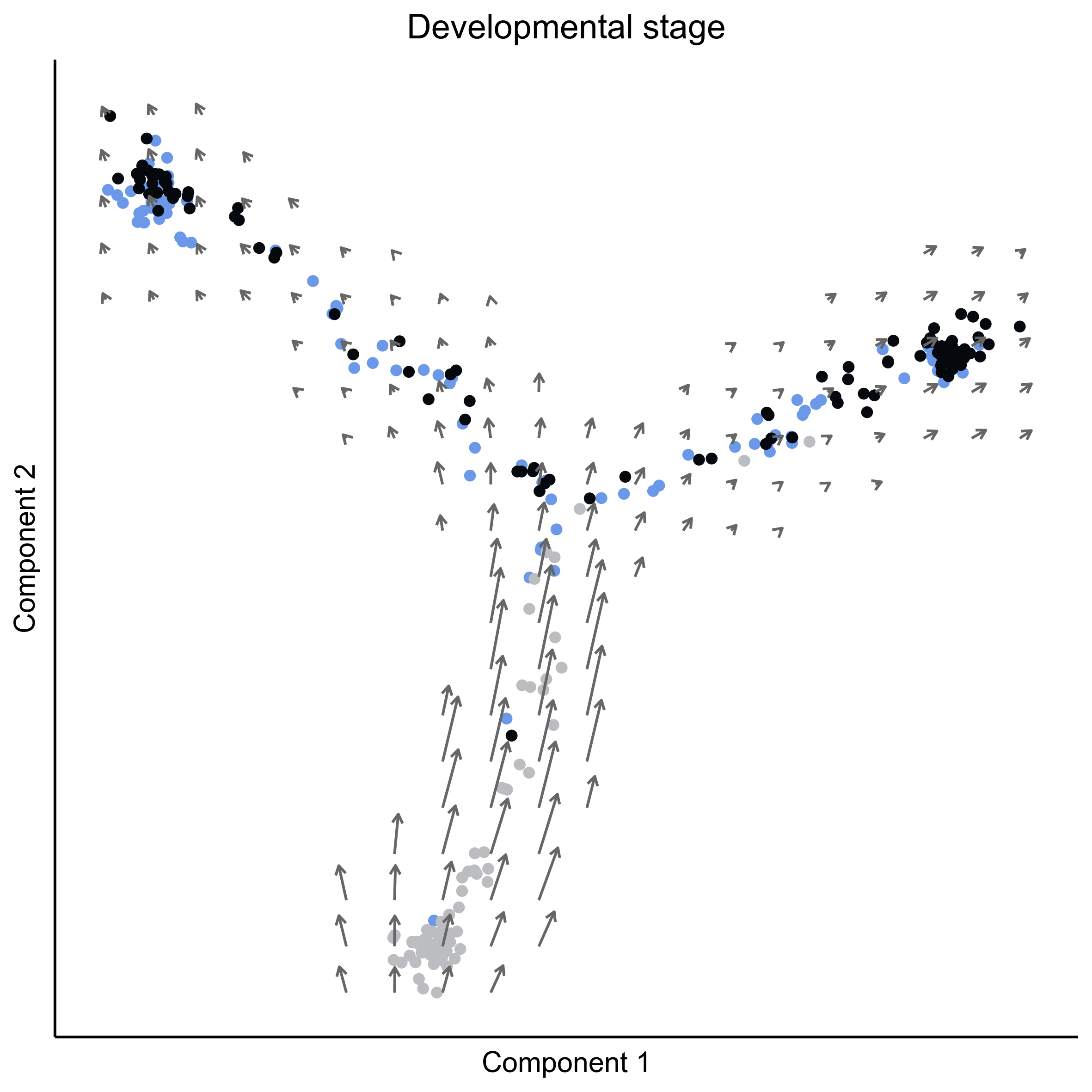
# plot cell arrows on stage
png(paste0(curr_plot_folder, 'Monocle_velocity_stage_arrows.png'), height = 15, width = 15, family = 'Arial', units = "cm", res = 400)
ggplot(data.frame('Component 1' = reducedDimS(HSMM)[1,], 'Component 2' = reducedDimS(HSMM)[2,],
'colour_by' = as.factor(pData(m_oep$expressionSet)$timepoint), check.names = FALSE), aes(x=`Component 1`, y=`Component 2`, color=colour_by)) +
geom_point() +
scale_color_manual(values = stage_cols) +
geom_segment(data = as.data.frame(vector_dat$arrows),
aes(x = x0, xend = x1, y = y0, yend = y1),
size = 0.5,
arrow = arrow(length = unit(4, "points"), type = "open"),
colour = "grey40") +
theme_classic() +
theme(legend.position = "none", axis.ticks=element_blank(), axis.text = element_blank()) +
ggtitle('Developmental stage') +
theme(plot.title = element_text(hjust = 0.5))
graphics.off()
×