Embryos at ss3-5 where electroporated with either Lmx1aE1-EGFP or Sox3U3-EGFP enhancers to genetically label the otic and epibranchial cell populations respectively. At ss18-21 embryos were removed from the egg and EGFP+ cells of each population were collected by FACS and processed for RNAseq.
Differential expression analysis is carried out using DESeq2 (Love et al. 2014).
Automatic switch for running pipeline through Nextflow or interactively in Rstudio.
library(getopt)
spec = matrix(c(
  'runtype', 'l', 2, "character",
  'cores'   , 'c', 2, "integer"
), byrow=TRUE, ncol=4)
opt = getopt(spec)

# Set run location
if(length(commandArgs(trailingOnly = TRUE)) == 0){
  cat('No command line arguments provided, user defaults paths are set for running interactively in Rstudio on docker\n')
  opt$runtype = "user"
} else {
  if(is.null(opt$runtype)){
    stop("--runtype must be either 'user' or 'nextflow'")
  }
  if(tolower(opt$runtype) != "user" & tolower(opt$runtype) != "nextflow"){
    stop("--runtype must be either 'user' or 'nextflow'")
  }
}
Set paths and load data and packages.
{
  if (opt$runtype == "user"){
    output_path = "./output/NF-downstream_analysis/lmx1a_dea/output/"
    input_file <- "./alignment_output/NF-lmx1a_alignment/featurecounts.merged.counts.tsv"

  } else if (opt$runtype == "nextflow"){
    cat('pipeline running through nextflow\n')

    output_path = "output/"
    input_file <- "./featurecounts.merged.counts.tsv"
  }

  dir.create(output_path, recursive = T)

  library(biomaRt)
  library(tidyverse)
  library(readr)
  library(RColorBrewer)
  library(VennDiagram)

  library(pheatmap)
  library(ggplot2)
  library(ggrepel)
  library(DESeq2)
  library(apeglm)
  library(openxlsx)
  library(extrafont)
}
Data pre-processing.
# read in count data and rename columns
read_counts <- read.delim(input_file, stringsAsFactors = FALSE)
colnames(read_counts)[1] <- "gene_id"

# if gene name exists then take gene name, else take ensembl ID and make new name column
read_counts <- read_counts %>% mutate(gene_name = ifelse(!is.na(gene_name), gene_name, gene_id))

# make duplicated gene names unique using "_"
read_counts$gene_name <- make.unique(read_counts$gene_name, sep = "_")

# make gene annotations dataframe
gene_annotations <- read_counts %>% dplyr::select(gene_id, gene_name)

# write CSV for output list
write.csv(read_counts, paste0(output_path, "read_counts.csv"), row.names = F)

# make rownames gene_id and remove ID and names column before making deseq object
rownames(read_counts) <- read_counts$gene_id
read_counts[,1:2] <- NULL
Run DESeq2.
### Add sample group to metadata
col_data <- as.data.frame(sapply(colnames(read_counts), function(x){ifelse(grepl("Lmx1a_E1", x), "Lmx1a_E1", "Sox3U3")}))
colnames(col_data) <- "Group"

### Make deseq object and make Sox3U3 group the reference level
deseq <- DESeqDataSetFromMatrix(read_counts, design = ~ Group, colData = col_data)
deseq$Group <- droplevels(deseq$Group)
deseq$Group <- relevel(deseq$Group, ref = "Sox3U3")

# set plot colours
plot_colours <- list(Group = c(Sox3U3 = "#48d1cc", Lmx1a_E1 = "#f55f20"))

### Filter genes which have fewer than 10 readcounts
deseq <- deseq[rowSums(counts(deseq)) >= 10, ]

### Run deseq test - size factors for normalisation during this step are calculated using median of ratios method
deseq <- DESeq(deseq)
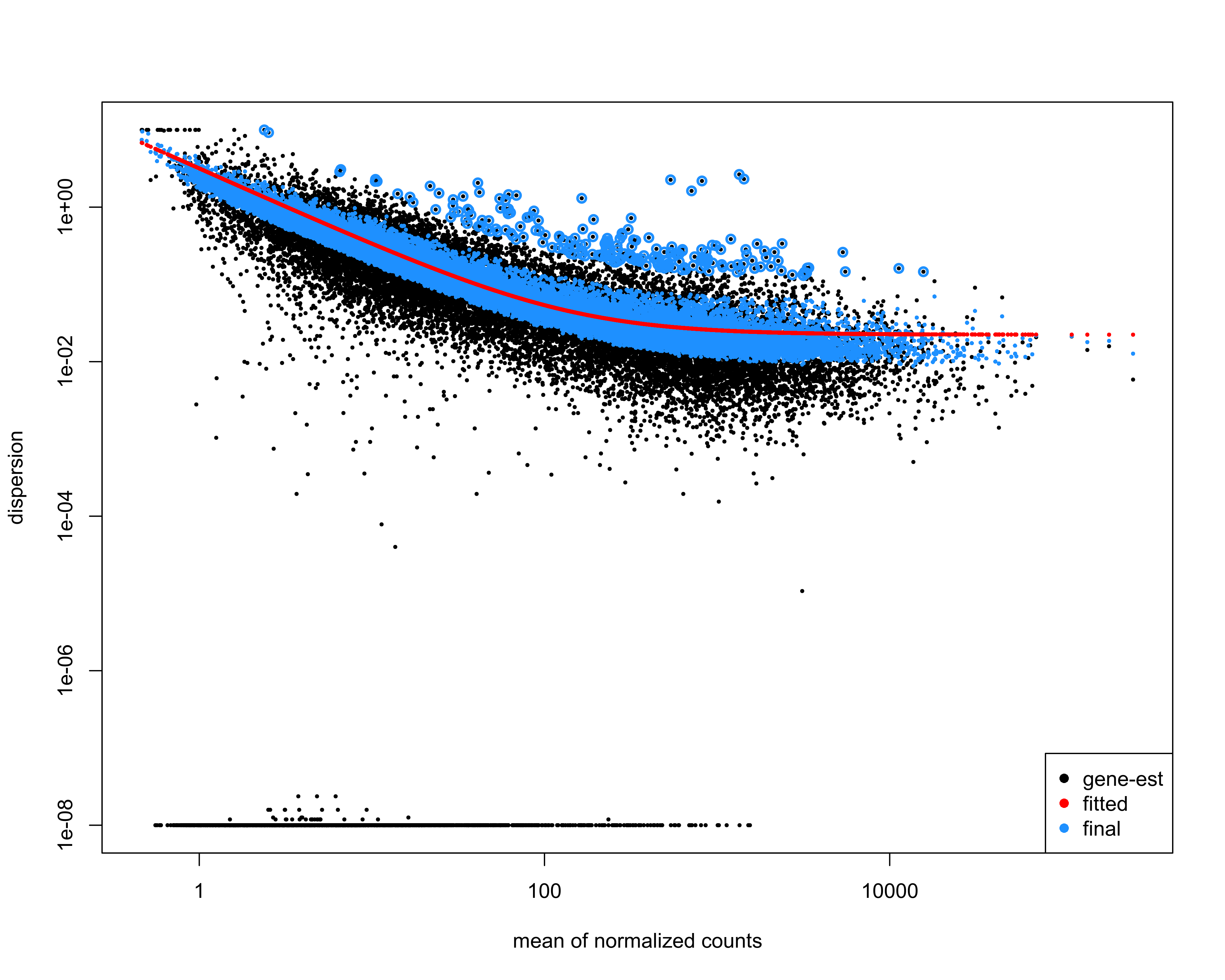
Plot dispersion estimates.
png(paste0(output_path, "dispersion_est.png"), height = 20, width = 25, family = 'Arial', units = "cm", res = 400)
plotDispEsts(deseq)
graphics.off()
We use the DESeq2 function lfcShrink in order to calculate more accurate log2FC estimates. This uses information across all genes to shrink LFC when a gene has low counts or high dispersion values.
# Run lfcShrink
res <- lfcShrink(deseq, coef="Group_Lmx1a_E1_vs_Sox3U3", type="apeglm")

# Add gene names to shrunken LFC dataframe
res$gene_name <- gene_annotations$gene_name[match(rownames(res), gene_annotations$gene_id)]
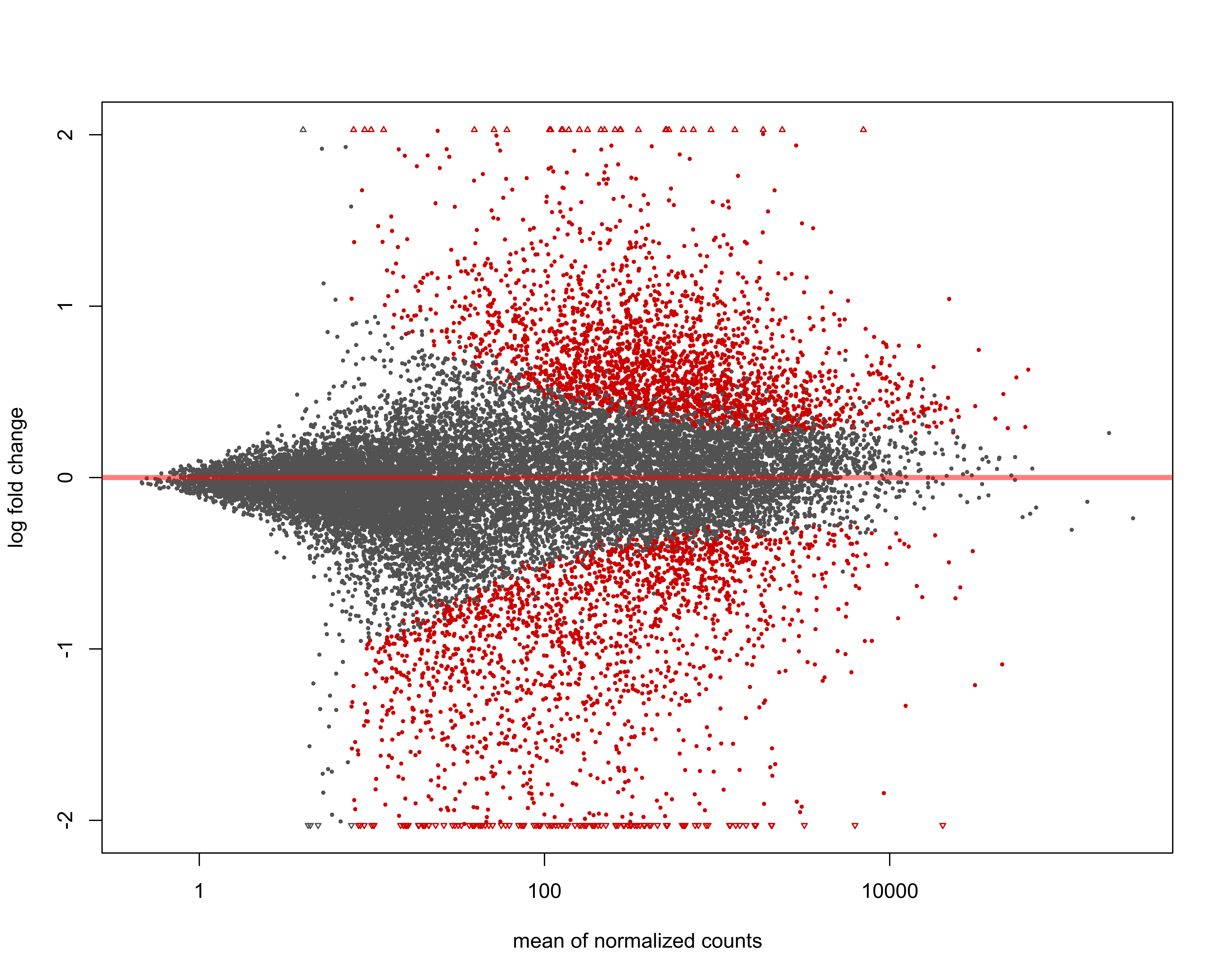
Plot MA with cutoff for significant genes = padj < 0.05.
png(paste0(output_path, "MA_plot.png"), height = 20, width = 25, family = 'Arial', units = "cm", res = 400)
DESeq2::plotMA(res, alpha = 0.05)
graphics.off()
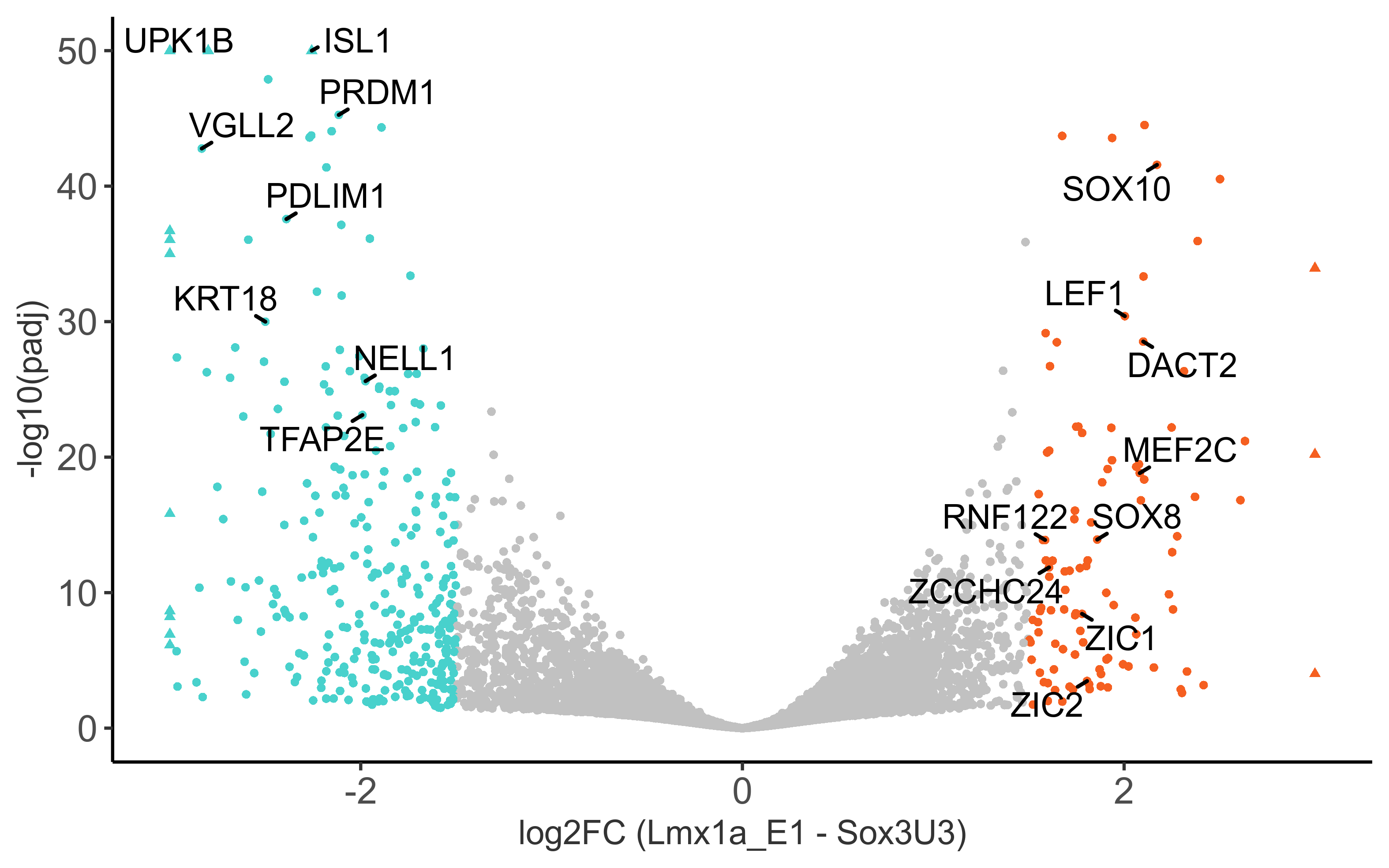
Plot volcano plot with padj < 0.05 and abs(fold change) > 1.5.
volc_dat <- as.data.frame(res[,-6])

# add gene name to volcano data
volc_dat$gene <- gene_annotations$gene_name[match(rownames(volc_dat), gene_annotations$gene_id)]

# label significance
volc_dat <- volc_dat %>%
  filter(!is.na(padj)) %>%
  mutate(sig = case_when((padj < 0.05 & log2FoldChange > 1.5) == 'TRUE' ~ 'upregulated',
                         (padj < 0.05 & log2FoldChange < -1.5) == 'TRUE' ~ 'downregulated',
                         (padj >= 0.05 | abs(log2FoldChange) <= 1.5) == 'TRUE' ~ 'not sig')) %>%
  arrange(abs(padj))

# label outliers with triangles for volcano plot
volc_dat <- volc_dat %>%
  mutate(shape = ifelse(abs(log2FoldChange) > 3 | -log10(padj) > 50, "triangle", "circle")) %>%
  mutate(log2FoldChange = ifelse(log2FoldChange > 3, 3, log2FoldChange)) %>%
  mutate(log2FoldChange = ifelse(log2FoldChange < -3, -3, log2FoldChange)) %>%
  mutate('-log10(padj)' = ifelse(-log10(padj) > 50, 50, -log10(padj)))


# select genes to add as labels on volcano plot
otic_genes <- c('MEF2C', 'SOX10', 'SOX8', 'ZIC1', 'ZIC2', 'DACT2', 'LEF1', 'ZCCHC24', 'RNF122')
epibranchial_genes <- c('PRDM1', 'VGLL2', 'PDLIM1', 'KRT18', 'ISL1', 'UPK1B', 'TFAP2E', 'NELL1')

png(paste0(output_path, "volcano.png"), width = 11.5, height = 7, family = 'Arial', units = "cm", res = 500)
ggplot(volc_dat, aes(log2FoldChange, `-log10(padj)`, shape=shape, label = gene)) +
  geom_point(aes(colour = sig, fill = sig), size = 1) +
  scale_fill_manual(breaks = c("not sig", "downregulated", "upregulated"),
                    values = alpha(c(plot_colours$Group[1], "#c1c1c1", plot_colours$Group[2]), 0.3)) +
  scale_color_manual(breaks = c("not sig", "downregulated", "upregulated"),
                     values= c(plot_colours$Group[1], "#c1c1c1", plot_colours$Group[2])) +
  theme(panel.grid.major = element_blank(), panel.grid.minor = element_blank(),
        panel.background = element_blank(), axis.line = element_line(colour = "black"),
        text = element_text(family = "", color = "grey20"),
        legend.position = "none", legend.title = element_blank()) +
  geom_text_repel(data = subset(volc_dat, gene %in% c(otic_genes, epibranchial_genes)), min.segment.length = 0, segment.size  = 0.6, segment.color = "black") +
  xlab('log2FC (Lmx1a_E1 - Sox3U3)') +
  theme(legend.position = "none")
graphics.off()
Generate csv for raw counts, normalised counts, and differential expression output.
# raw counts dataframe
raw_counts <- as.data.frame(counts(deseq))
colnames(raw_counts) <- paste0("counts_", colnames(raw_counts))
raw_counts$gene_id <- rownames(raw_counts)

# normalised counts dataframe
norm_counts <- as.data.frame(counts(deseq, normalized=TRUE))
colnames(norm_counts) <- paste0("norm_size.adj_", colnames(norm_counts))
norm_counts$gene_id <- rownames(norm_counts)

# differential expression statistics dataframe
DE_res <- as.data.frame(res)
DE_res$gene_id <- rownames(DE_res)

# merge raw_counts, norm_counts and DE_res together into a single dataframe
all_dat <- merge(raw_counts, norm_counts, by = 'gene_id')
all_dat <- merge(all_dat, DE_res, by = 'gene_id')

# move position of gene names column
all_dat <- all_dat[,c(1, ncol(all_dat), 2:{ncol(all_dat)-1})]

# Find which genes are up and downregulated following differential expression analysis
res_up <- all_dat[which(all_dat$padj < 0.05 & all_dat$log2FoldChange > 1.5), ]
res_up <- res_up[order(-res_up$log2FoldChange),]

res_down <- all_dat[which(all_dat$padj < 0.05 & all_dat$log2FoldChange < -1.5), ]
res_down <- res_down[order(res_down$log2FoldChange),]

nrow(res_up)
nrow(res_down)
# 422 genes DE with padj 0.05 & abs(logFC) > 1.5 (103 upregulated, 319 downregulated)


# Write DE data as a csv
res_de <- rbind(res_up, res_down) %>% arrange(-log2FoldChange)

cat("This table shows the differential expression results for genes with absolute log2FC > 1.5 and adjusted p-value < 0.05 when comparing Lmx1a_E1 and Sox3U3 samples (Lmx1a_E1 - Sox3U3)
Reads are aligned to Galgal6 \n
Statistics:
Normalised count: read counts adjusted for library size
pvalue: unadjusted pvalue for differential expression test between Lmx1a_E1 and Sox3U3 samples
padj: pvalue for differential expression test between Lmx1a_E1 and Sox3U3 samples - adjusted for multiple testing (Benjamini and Hochberg) \n \n",
    file = paste0(output_path, "Lmx1a_E1_SupplementaryData_1.csv"))
write.table(res_de, paste0(output_path, "Lmx1a_E1_SupplementaryData_1.csv"), append=TRUE, row.names = F, na = 'NA', sep=",")


# non-DE genes
res_remain <- all_dat[!rownames(all_dat) %in% rownames(res_up) & !rownames(all_dat) %in% rownames(res_down),]
res_remain <- res_remain[order(-res_remain$log2FoldChange),]

# Make a single dataframe with ordered rows
all_dat <- rbind(res_up, res_down, res_remain)

# Write all data as a csv
cat("This table shows the differential expression results for all genes when comparing Lmx1a_E1 and Sox3U3 samples (Lmx1a_E1 - Sox3U3)
Reads are aligned to Galgal6 \n
Statistics:
Normalised count: read counts adjusted for library size
pvalue: unadjusted pvalue for differential expression test between Lmx1a_E1 and Sox3U3 samples
padj: pvalue for differential expression test between Lmx1a_E1 and Sox3U3 samples - adjusted for multiple testing (Benjamini and Hochberg) \n \n",
    file = paste0(output_path, "Lmx1a_E1_process_output_1.csv"))
write.table(all_dat, paste0(output_path, "Lmx1a_E1_process_output_1.csv"), append=TRUE, row.names = F, na = 'NA', sep=",")
Download differential expression results for all genes.
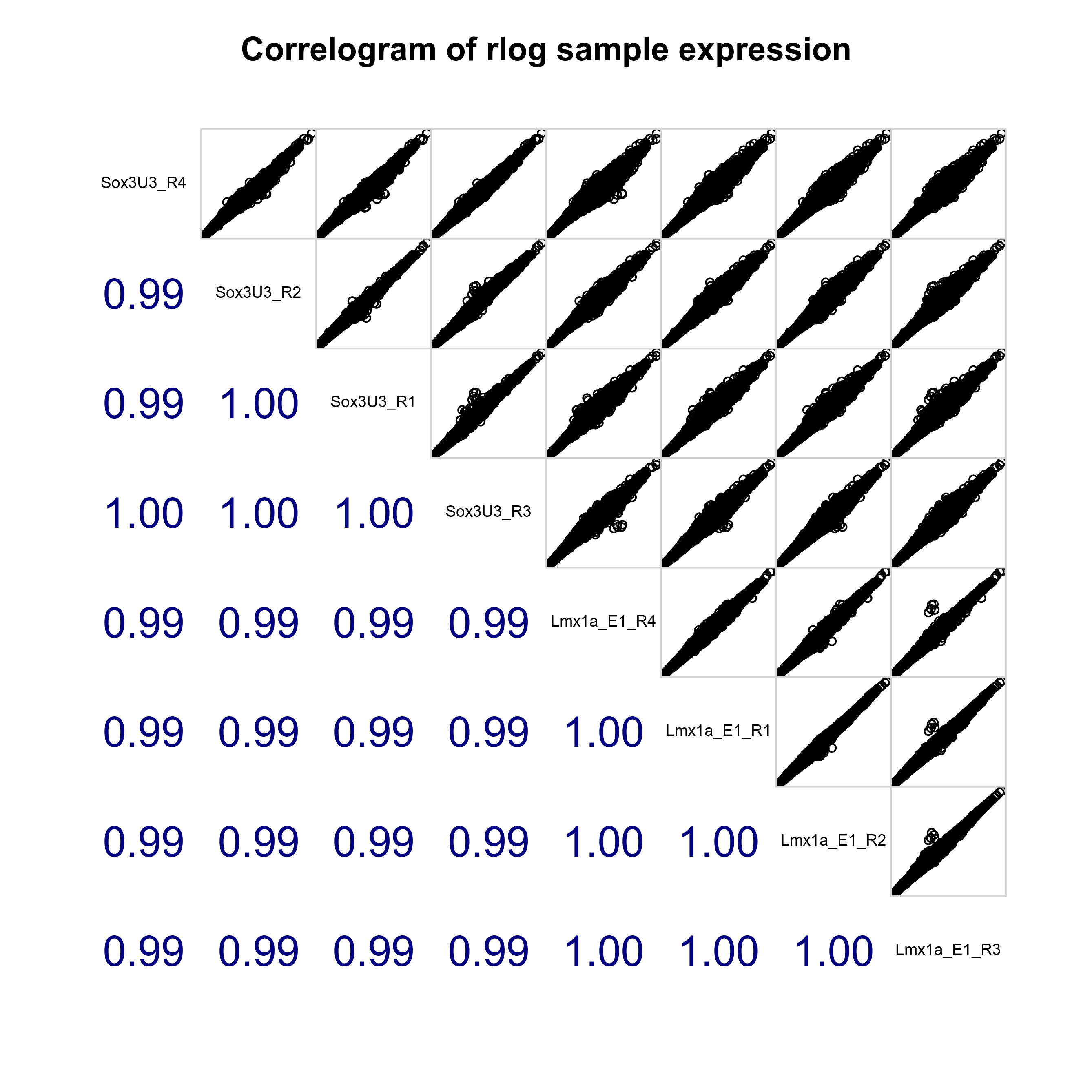
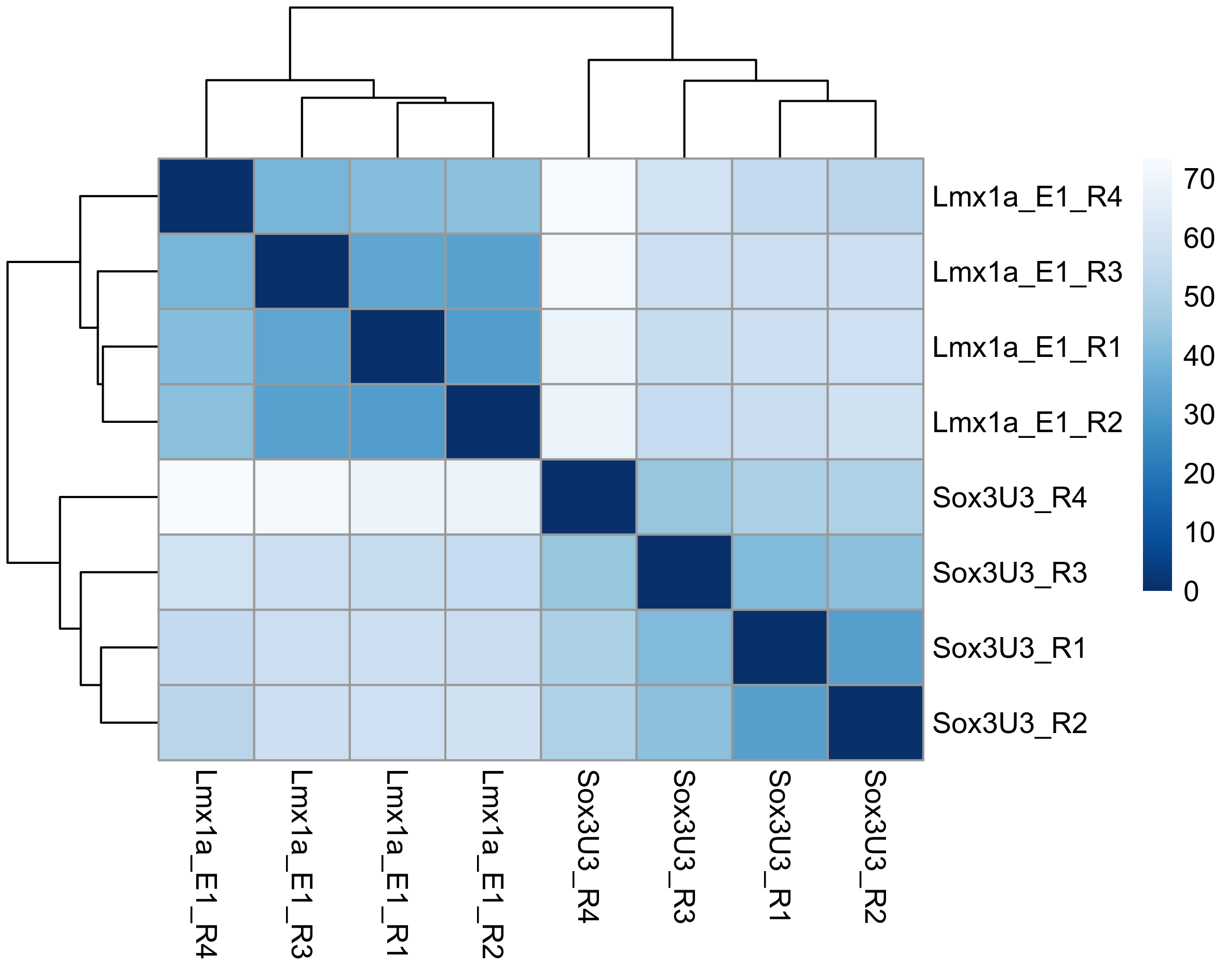
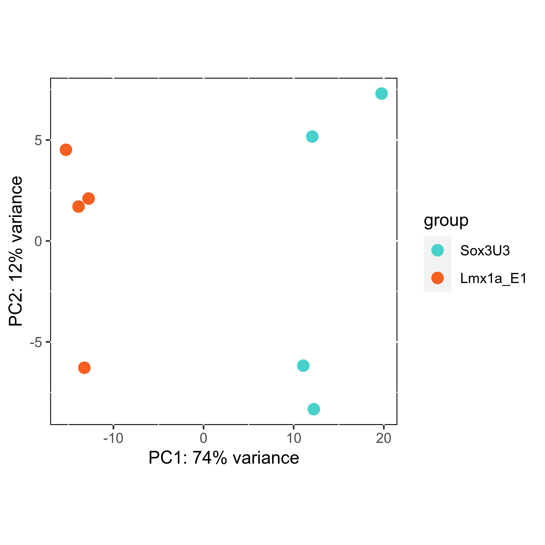
Plot sample-sample distances, PCA plot and correlogram to show relationship between samples.
# To prevent the highest expressed genes from dominating when clustering we need to rlog (regularised log) transform the data
rld <- rlog(deseq, blind=FALSE)

# Plot sample correlogram
png(paste0(output_path, "SampleCorrelogram.png"), height = 17, width = 17, family = 'Arial', units = "cm", res = 400)
corrgram::corrgram(as.data.frame(assay(rld)), order=TRUE, lower.panel=corrgram::panel.cor,
                   upper.panel=corrgram::panel.pts, text.panel=corrgram::panel.txt,
                   main="Correlogram of rlog sample expression", cor.method = 'pearson')
graphics.off()

# Plot sample distance heatmap
sample_dists <- dist(t(assay(rld)))

sampleDistMatrix <- as.matrix(sample_dists)
rownames(sampleDistMatrix) <- paste(colnames(rld))
colnames(sampleDistMatrix) <- paste(colnames(rld))
colours = colorRampPalette(rev(brewer.pal(9, "Blues")))(255)

png(paste0(output_path, "SampleDist.png"), height = 12, width = 15, family = 'Arial', units = "cm", res = 400)
pheatmap(sampleDistMatrix, color = colours)
graphics.off()

# Plot sample PCA
png(paste0(output_path, "SamplePCA.png"), height = 12, width = 12, family = 'Arial', units = "cm", res = 400)
plotPCA(rld, intgroup = "Group") +
  scale_color_manual(values=plot_colours$Group) +
  theme(aspect.ratio=1,
        panel.background = element_rect(fill = "white", colour = "black"))
graphics.off()
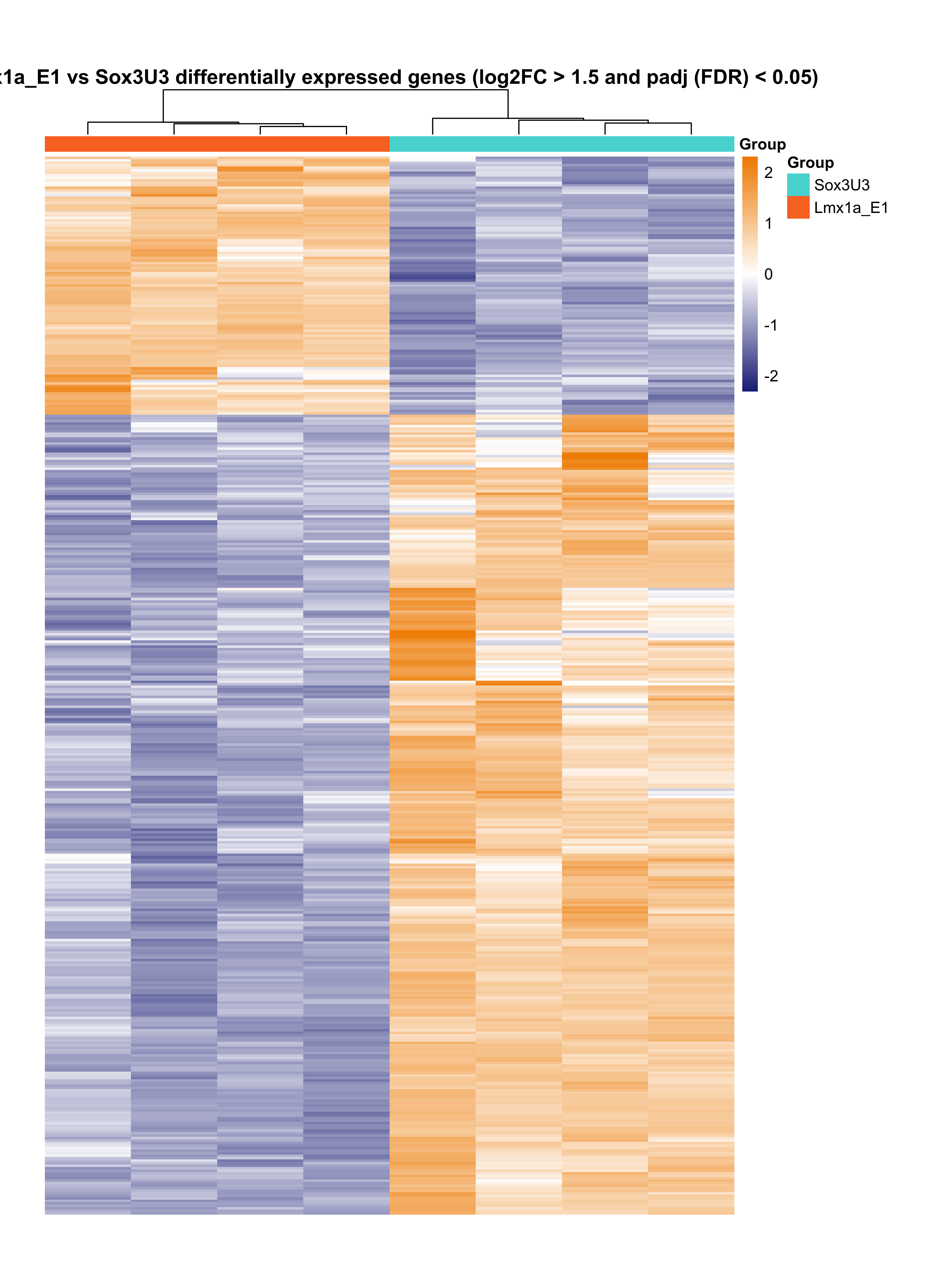
Subset differentially expressed genes (adjusted p-value < 0.05, absolute log2FC > 1.5).
res_sub <- res[which(res$padj < 0.05 & abs(res$log2FoldChange) > 1.5), ]
res_sub <- res_sub[order(-res_sub$log2FoldChange),]
Plot heatmap of differentially expressed genes.
png(paste0(output_path, "Lmx1a_E1_hm.png"), height = 29, width = 21, family = 'Arial', units = "cm", res = 400)
pheatmap(assay(rld)[rownames(res_sub),], color = colorRampPalette(c("#191d73", "white", "#ed7901"))(n = 100), cluster_rows=T, show_rownames=FALSE,
         show_colnames = F, cluster_cols=T, annotation_col=as.data.frame(colData(deseq)["Group"]),
         annotation_colors = plot_colours, scale = "row", treeheight_row = 0, treeheight_col = 25,
         main = "Lmx1a_E1 vs Sox3U3 differentially expressed genes (log2FC > 1.5 and padj (FDR) < 0.05)", border_color = NA, cellheight = 1.6, cellwidth = 55)
graphics.off()
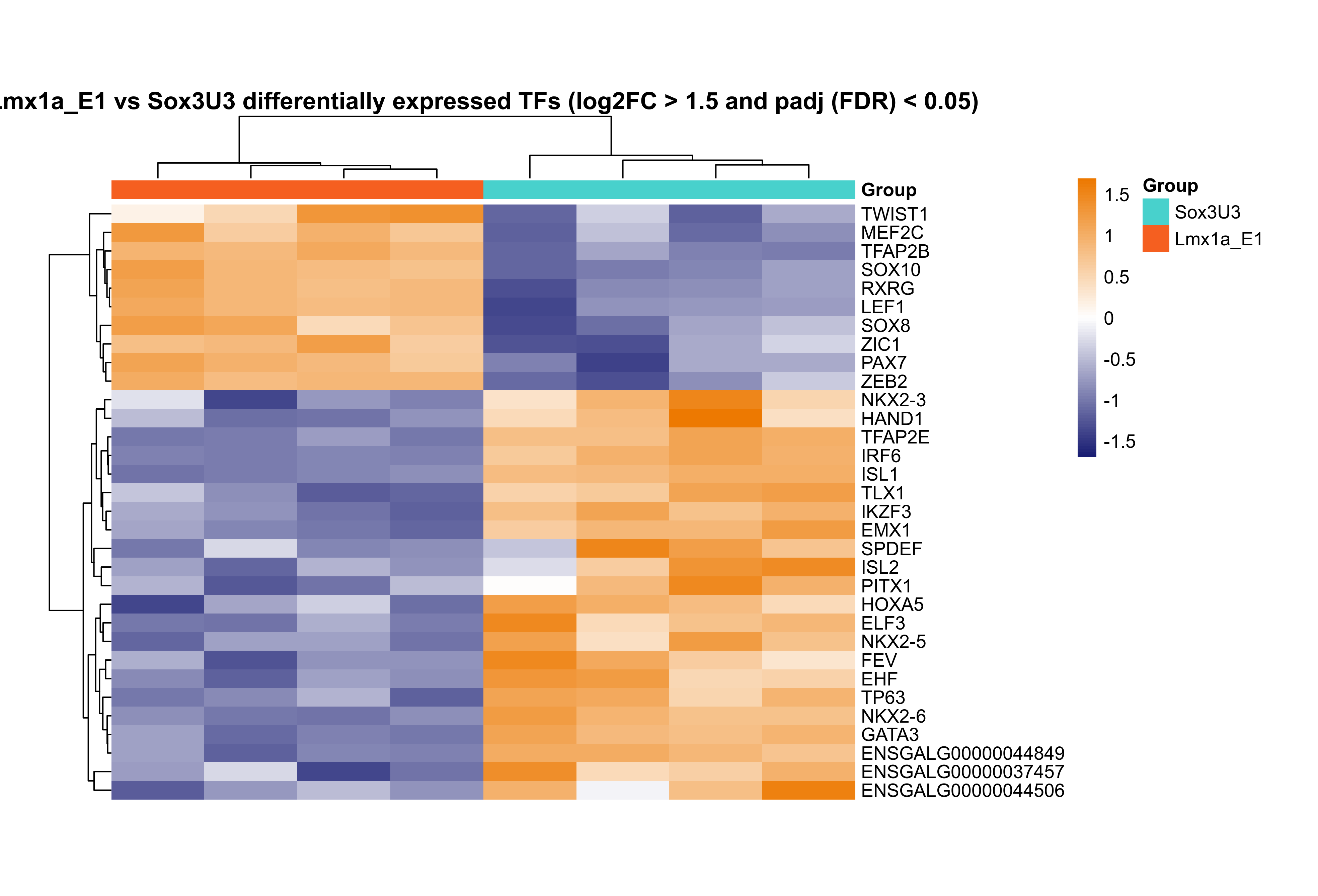
Subset differentially expressed transcription factors based on GO terms ('GO:0003700', 'GO:0043565', 'GO:0000981').
# Get biomart GO annotations for TFs
ensembl <- useEnsembl(biomart = 'ensembl',
                      dataset = 'ggallus_gene_ensembl',
                      version = 104)

TF_subset <- getBM(attributes=c("ensembl_gene_id", "go_id", "name_1006", "namespace_1003"),
                   filters = 'ensembl_gene_id',
                   values = rownames(res_sub),
                   mart = ensembl)

# subset genes based on transcription factor GO terms
TF_subset <- TF_subset$ensembl_gene_id[TF_subset$go_id %in% c('GO:0003700', 'GO:0043565', 'GO:0000981')]

res_sub_TF <- res_sub[rownames(res_sub) %in% TF_subset,]
Generate csv for raw counts, normalised counts, and differential expression output for transcription factors.
# subset TFs from all_dat
all_dat_TF <- all_dat[all_dat$gene_id %in% rownames(res_sub_TF),]

cat("This table shows differentially expressed (absolute FC > 1.5 and padj (FDR) < 0.05) transcription factors between Lmx1a_E1 and Sox3U3 samples (Lmx1a_E1 - Sox3U3)
Reads are aligned to Galgal6 \n
Statistics:
Normalised count: read counts adjusted for library size
pvalue: unadjusted pvalue for differential expression test between Lmx1a_E1 and Sox3U3 samples
padj: pvalue for differential expression test between Lmx1a_E1 and Sox3U3 samples - adjusted for multiple testing (Benjamini and Hochberg) \n \n",
    file = paste0(output_path, "Lmx1a_E1_process_output_2.csv"))
write.table(all_dat_TF, paste0(output_path, "Lmx1a_E1_process_output_2.csv"), append=TRUE, row.names = F, na = 'NA', sep=",")
Download TF differential expression results (absolute log2FC > 1.5 and adjusted p-value < 0.05).
Plot heatmap for differentially expressed transcription factors.
rld.plot <- assay(rld)
rownames(rld.plot) <- gene_annotations$gene_name[match(rownames(rld.plot), gene_annotations$gene_id)]

# plot DE TFs
png(paste0(output_path, "Lmx1a_E1_TFs_hm.png"), height = 17, width = 25, family = 'Arial', units = "cm", res = 400)
pheatmap(rld.plot[res_sub_TF$gene_name,], color = colorRampPalette(c("#191d73", "white", "#ed7901"))(n = 100), cluster_rows=T, show_rownames=T,
         show_colnames = F, cluster_cols=T, treeheight_row = 30, treeheight_col = 30,
         annotation_col=as.data.frame(col_data["Group"]), annotation_colors = plot_colours,
         scale = "row", main = "Lmx1a_E1 vs Sox3U3 differentially expressed TFs (log2FC > 1.5 and padj (FDR) < 0.05)", border_color = NA, cellheight = 10, cellwidth = 50)
graphics.off()
×