In order to study if Sox8 overexpression can confer otic characer, we co-electroporated a combination of Sox8-mCherry and Lmx1aE1-EGFP (Sox8OE) or constitutive mCherry and EGFP (Control), at head fold stages. Then, at ss12-13, we collected double positive cells of the cranial ectoderm by FACS (heads of embryos were dissected rostral to the otic placode, leaving the otic placode and trunk tissue behind) and processed them for RNAseq.
Differential expression analysis is carried out using DESeq2 (Love et al. 2014).
Automatic switch for running pipeline through Nextflow or interactively in Rstudio.
library(getopt)
spec = matrix(c(
  'runtype', 'l', 2, "character",
  'cores'   , 'c', 2, "integer"
), byrow=TRUE, ncol=4)
opt = getopt(spec)

# Set run location
if(length(commandArgs(trailingOnly = TRUE)) == 0){
  cat('No command line arguments provided, user defaults paths are set for running interactively in Rstudio on docker\n')
  opt$runtype = "user"
} else {
  if(is.null(opt$runtype)){
    stop("--runtype must be either 'user' or 'nextflow'")
  }
  if(tolower(opt$runtype) != "user" & tolower(opt$runtype) != "nextflow"){
    stop("--runtype must be either 'user' or 'nextflow'")
  }
}
Set paths and load data and packages.
{
  if (opt$runtype == "user"){
    output_path = "./output/NF-downstream_analysis/sox8_dea/output/"
    input_file <- "./alignment_output/NF-sox8_alignment/featurecounts.merged.counts.tsv"

  } else if (opt$runtype == "nextflow"){
    cat('pipeline running through nextflow\n')

    output_path = "output/"
    input_file <- "./featurecounts.merged.counts.tsv"
  }

  dir.create(output_path, recursive = T)

  library(biomaRt)
  library(tidyverse)
  library(readr)
  library(RColorBrewer)
  library(VennDiagram)

  library(pheatmap)
  library(ggplot2)
  library(ggrepel)
  library(DESeq2)
  library(apeglm)
  library(openxlsx)
  library(corrgram)
  library(extrafont)
}
Data pre-processing.
# read in count data and rename columns
read_counts <- read.delim(input_file, stringsAsFactors = FALSE)
colnames(read_counts)[1] <- "gene_id"

# if gene name exists then take gene name, else take ensembl ID and make new name column
read_counts <- read_counts %>% mutate(gene_name = ifelse(!is.na(gene_name), gene_name, gene_id))

# make duplicated gene names unique using "_"
read_counts$gene_name <- make.unique(read_counts$gene_name, sep = "_")

# make gene annotations dataframe
gene_annotations <- read_counts %>% dplyr::select(gene_id, gene_name)

# write CSV for output list
write.csv(read_counts, paste0(output_path, "read_counts.csv"), row.names = F)

# make rownames gene_id and remove ID and names column before making deseq object
rownames(read_counts) <- read_counts$gene_id
read_counts[,1:2] <- NULL
Run DESeq2.
# Add sample group to metadata
col_data <- as.data.frame(sapply(colnames(read_counts), function(x){ifelse(grepl("sox8_oe", x), "Sox8_OE", "Control")}))
colnames(col_data) <- "Group"

# Make deseq object and make Control group the reference level
deseq <- DESeqDataSetFromMatrix(read_counts, design = ~ Group, colData = col_data)
deseq$Group <- droplevels(deseq$Group)
deseq$Group <- relevel(deseq$Group, ref = "Control")

# set plot colours
plot_colours <- list(Group = c(Sox8_OE = "#f55f20", Control = "#957dad"))


# Filter genes which have fewer than 10 readcounts
deseq <- deseq[rowSums(counts(deseq)) >= 10, ]

# Run deseq test - size factors for normalisation during this step are calculated using median of ratios method
deseq <- DESeq(deseq)
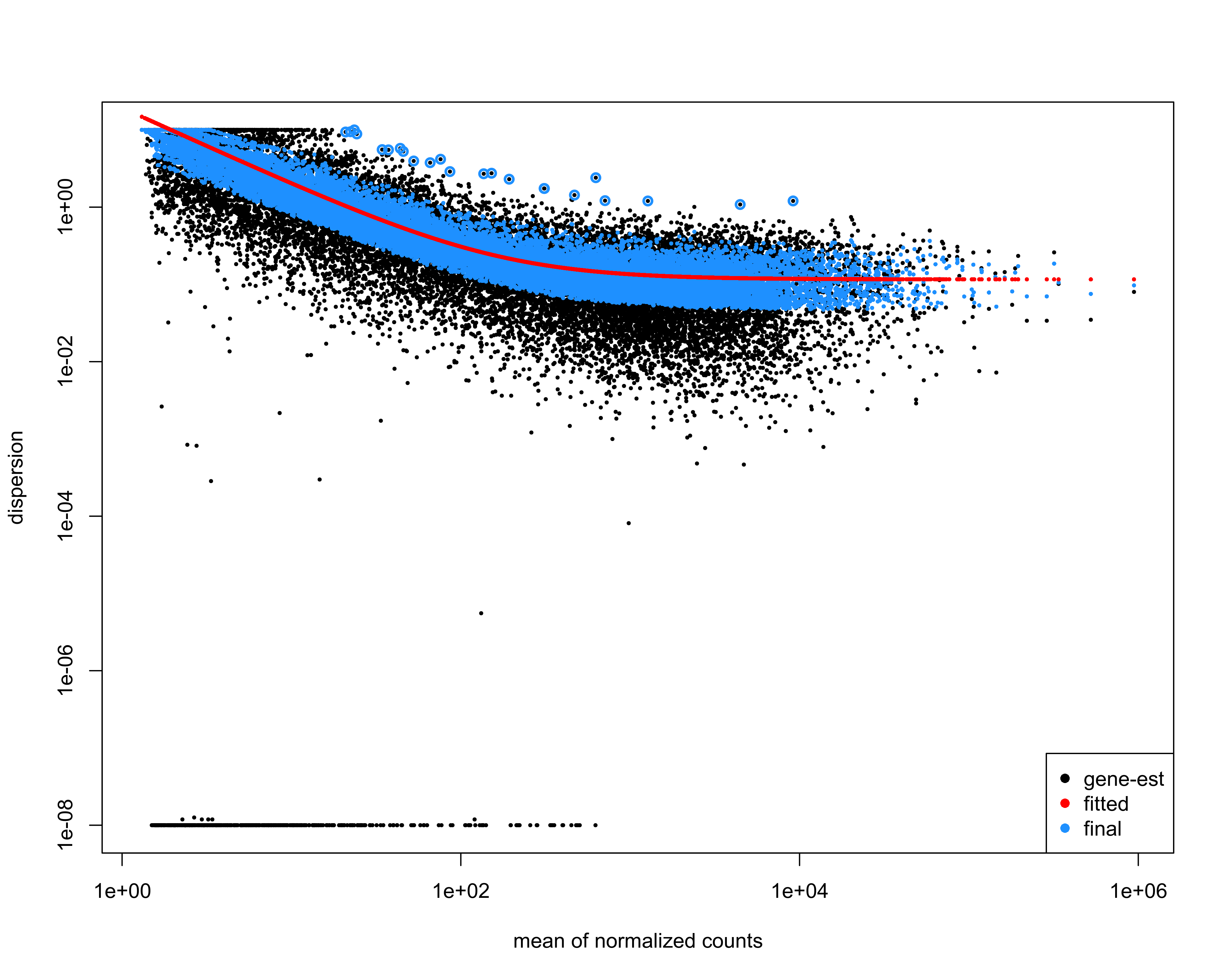
Plot dispersion estimates.
png(paste0(output_path, "dispersion_est.png"), height = 20, width = 25, family = 'Arial', units = "cm", res = 400)
plotDispEsts(deseq)
graphics.off()
We use the DESeq2 function lfcShrink in order to calculate more accurate log2FC estimates. This uses information across all genes to shrink LFC when a gene has low counts or high dispersion values.
# Run lfcShrink
res <- lfcShrink(deseq, coef="Group_Sox8_OE_vs_Control", type="apeglm")

# Add gene names to shrunken LFC dataframe
res$gene_name <- gene_annotations$gene_name[match(rownames(res), gene_annotations$gene_id)]
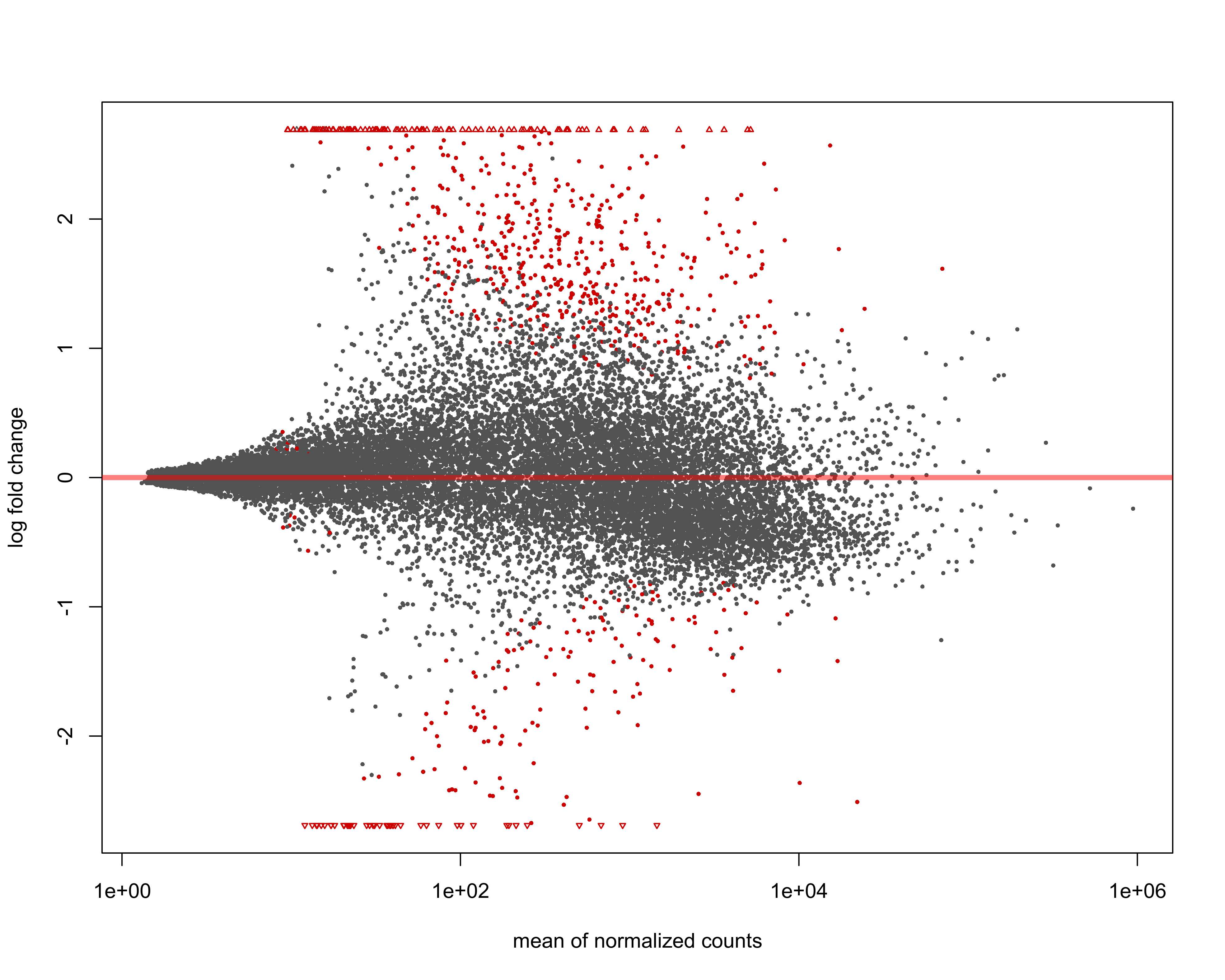
Plot MA with cutoff for significant genes = padj < 0.05
png(paste0(output_path, "MA_plot.png"), height = 20, width = 25, family = 'Arial', units = "cm", res = 400)
DESeq2::plotMA(res, alpha = 0.05)
graphics.off()
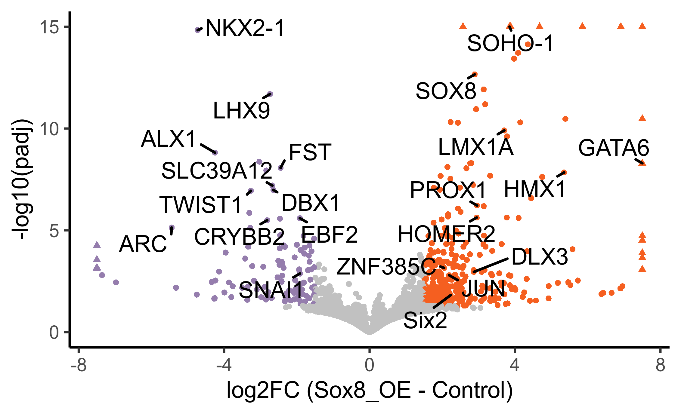
Plot volcano plot with padj < 0.05 and abs(fold change) > 1.5.
volc_dat <- as.data.frame(res[,-6])

# add gene name to volcano data
volc_dat$gene <- gene_annotations$gene_name[match(rownames(volc_dat), gene_annotations$gene_id)]

# label significance
volc_dat <- volc_dat %>%
  filter(!is.na(padj)) %>%
  mutate(sig = case_when((padj < 0.05 & log2FoldChange > 1.5) == 'TRUE' ~ 'upregulated',
                         (padj < 0.05 & log2FoldChange < -1.5) == 'TRUE' ~ 'downregulated',
                         (padj >= 0.05 | abs(log2FoldChange) <= 1.5) == 'TRUE' ~ 'not sig')) %>%
  arrange(abs(padj))

# label outliers with triangles for volcano plot
volc_dat <- volc_dat %>%
  mutate(shape = ifelse(abs(log2FoldChange)>7.5 | -log10(padj) > 15, "triangle", "circle")) %>%
  mutate(log2FoldChange = ifelse(log2FoldChange > 7.5, 7.5, log2FoldChange)) %>%
  mutate(log2FoldChange = ifelse(log2FoldChange < -7.5, -7.5, log2FoldChange)) %>%
  mutate('-log10(padj)' = ifelse(-log10(padj) > 15, 15, -log10(padj)))


# select genes to add as labels on volcano plot
otic_genes <- c("SOHO-1", "LMX1A", "SOX8", "HOMER2", "DLX3", "ZNF385C", "GATA6", "Six2", "JUN", "PROX1", "HMX1")

downreg <- volc_dat %>%
  dplyr::filter(log2FoldChange < 1.5) %>%
  dplyr::arrange(padj) %>%
  dplyr::mutate(gene = as.character(gene)) %>%
  dplyr::filter(!stringr::str_detect(gene, "ENS"))
downreg <- downreg[1:10,"gene"]

png(paste0(output_path, "volcano.png"), width = 16, height = 10, family = 'Arial', units = "cm", res = 500)
ggplot(volc_dat, aes(log2FoldChange, `-log10(padj)`, shape=shape, label = gene)) +
  geom_point(aes(colour = sig, fill = sig), size = 1) +
  scale_fill_manual(breaks = c("not sig", "downregulated", "upregulated"),
                    values = alpha(c(plot_colours$Group[2], "#c1c1c1", plot_colours$Group[1]), 0.3)) +
  scale_color_manual(breaks = c("not sig", "downregulated", "upregulated"),
                     values= c(plot_colours$Group[2], "#c1c1c1", plot_colours$Group[1])) +
  theme(panel.grid.major = element_blank(), panel.grid.minor = element_blank(),
        panel.background = element_blank(), axis.line = element_line(colour = "black"),
        legend.position = "none", legend.title = element_blank(),
        axis.text = element_text(size = 12)) +
  geom_text_repel(data = subset(volc_dat, gene %in% c(otic_genes, downreg, "SNAI1")), min.segment.length = 0, segment.size  = 0.6, segment.color = "black") +
  xlab('log2FC (Sox8_OE - Control)')
graphics.off()
Generate csv for raw counts, normalised counts, and differential expression output.
# raw counts dataframe
raw_counts <- as.data.frame(counts(deseq))
colnames(raw_counts) <- paste0("counts_", colnames(raw_counts))
raw_counts$gene_id <- rownames(raw_counts)

# normalised counts dataframe
norm_counts <- as.data.frame(counts(deseq, normalized=TRUE))
colnames(norm_counts) <- paste0("norm_size.adj_", colnames(norm_counts))
norm_counts$gene_id <- rownames(norm_counts)

# differential expression statistics dataframe
DE_res <- as.data.frame(res)
DE_res$gene_id <- rownames(DE_res)

# merge raw_counts, norm_counts and DE_res together into a single dataframe
all_dat <- merge(raw_counts, norm_counts, by = 'gene_id')
all_dat <- merge(all_dat, DE_res, by = 'gene_id')

# move position of gene names column
all_dat <- all_dat[,c(1, ncol(all_dat), 2:{ncol(all_dat)-1})]

# Find which genes are up and downregulated following differential expression analysis
res_up <- all_dat[which(all_dat$padj < 0.05 & all_dat$log2FoldChange > 1.5), ]
res_up <- res_up[order(-res_up$log2FoldChange),]

res_down <- all_dat[which(all_dat$padj < 0.05 & all_dat$log2FoldChange < -1.5), ]
res_down <- res_down[order(res_down$log2FoldChange),]

nrow(res_up)
nrow(res_down)
# 511 genes DE with padj 0.05 & abs(logFC) > 1.5 (399 upregulated, 112 downregulated)

# Write DE data as a csv
res_de <- rbind(res_up, res_down) %>% arrange(-log2FoldChange)

# Write all data as a csv
cat("This table shows the differential expression results for genes with absolute log2FC > 1.5 and adjusted p-value < 0.05 when comparing Sox8 overexpression and control samples (Sox8 - Control)
Reads are aligned to Galgal6 \n
Statistics:
Normalised count: read counts adjusted for library size
pvalue: unadjusted pvalue for differential expression test between Sox8 overexpression and control samples
padj: pvalue for differential expression test between Sox8 overexpression and control samples - adjusted for multiple testing (Benjamini and Hochberg) \n \n",
    file = paste0(output_path, "Sox8_OE_SupplementaryData_5.csv"))
write.table(res_de, paste0(output_path, "Sox8_OE_SupplementaryData_5.csv"), append=TRUE, row.names = F, na = 'NA', sep=",")


# non-DE genes
res_remain <- all_dat[!rownames(all_dat) %in% rownames(res_up) & !rownames(all_dat) %in% rownames(res_down),]
res_remain <- res_remain[order(-res_remain$log2FoldChange),]

# Make a single dataframe with ordered rows
all_dat <- rbind(res_up, res_down, res_remain)

# Write all data as a csv
cat("This table shows the differential expression results for all genes when comparing Sox8 overexpression and control samples (Sox8 - Control)
Reads are aligned to Galgal6 \n
Statistics:
Normalised count: read counts adjusted for library size
pvalue: unadjusted pvalue for differential expression test between Sox8 overexpression and control samples
padj: pvalue for differential expression test between Sox8 overexpression and control samples - adjusted for multiple testing (Benjamini and Hochberg) \n \n",
    file = paste0(output_path, "Sox8_OE_process_output_1.csv"))
write.table(all_dat, paste0(output_path, "Sox8_OE_process_output_1.csv"), append=TRUE, row.names = F, na = 'NA', sep=",")
Download differential expression results for all genes.
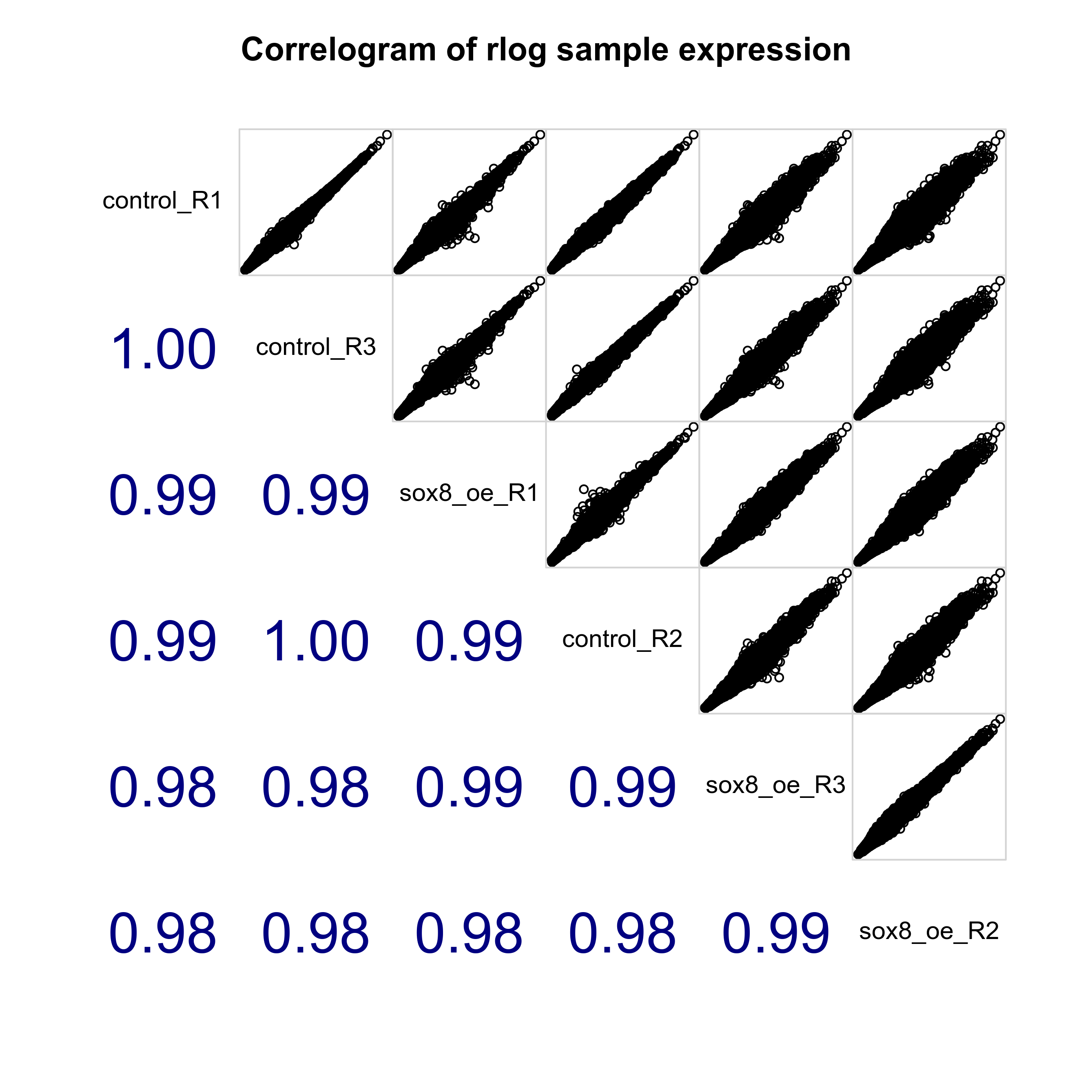
Plot sample-sample distances, PCA plot and correlogram to show relationship between samples.
# To prevent the highest expressed genes from dominating when clustering we need to rlog (regularised log) transform the data
rld <- rlog(deseq, blind=FALSE)
# Plot sample correlogram
png(paste0(output_path, "SampleCorrelogram.png"), height = 17, width = 17, family = 'Arial', units = "cm", res = 400)
corrgram::corrgram(as.data.frame(assay(rld)), order=TRUE, lower.panel=corrgram::panel.cor,
upper.panel=corrgram::panel.pts, text.panel=corrgram::panel.txt,
main="Correlogram of rlog sample expression", cor.method = 'pearson')
graphics.off()
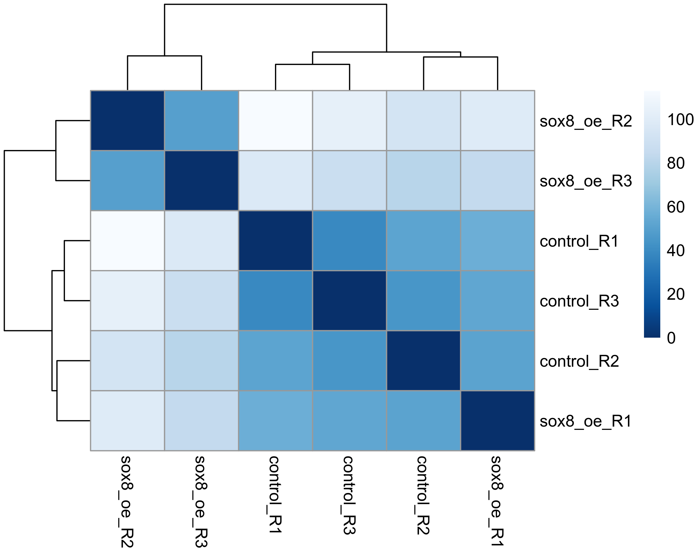
# Plot sample distance heatmap
sample_dists <- dist(t(assay(rld)))
sampleDistMatrix <- as.matrix(sample_dists)
rownames(sampleDistMatrix) <- paste(colnames(rld))
colnames(sampleDistMatrix) <- paste(colnames(rld))
colours = colorRampPalette(rev(brewer.pal(9, "Blues")))(255)
png(paste0(output_path, "SampleDist.png"), height = 12, width = 15, family = 'Arial', units = "cm", res = 400)
pheatmap(sampleDistMatrix, color = colours)
graphics.off()
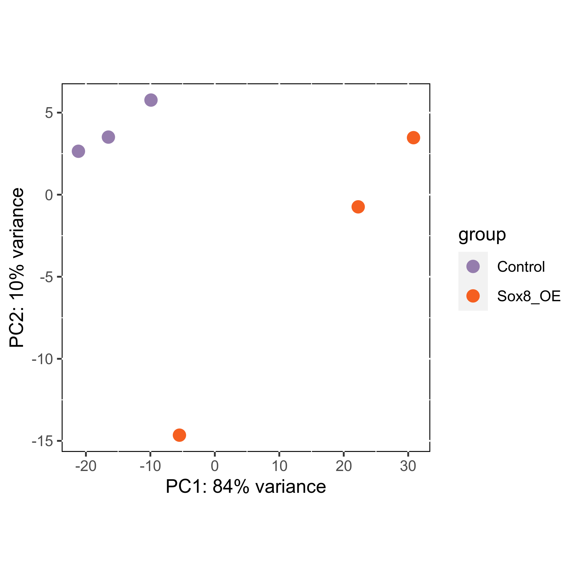
# Plot sample PCA
png(paste0(output_path, "SamplePCA.png"), height = 12, width = 12, family = 'Arial', units = "cm", res = 400)
plotPCA(rld, intgroup = "Group") +
scale_color_manual(values=plot_colours$Group) +
theme(aspect.ratio=1,
panel.background = element_rect(fill = "white", colour = "black"))
graphics.off()
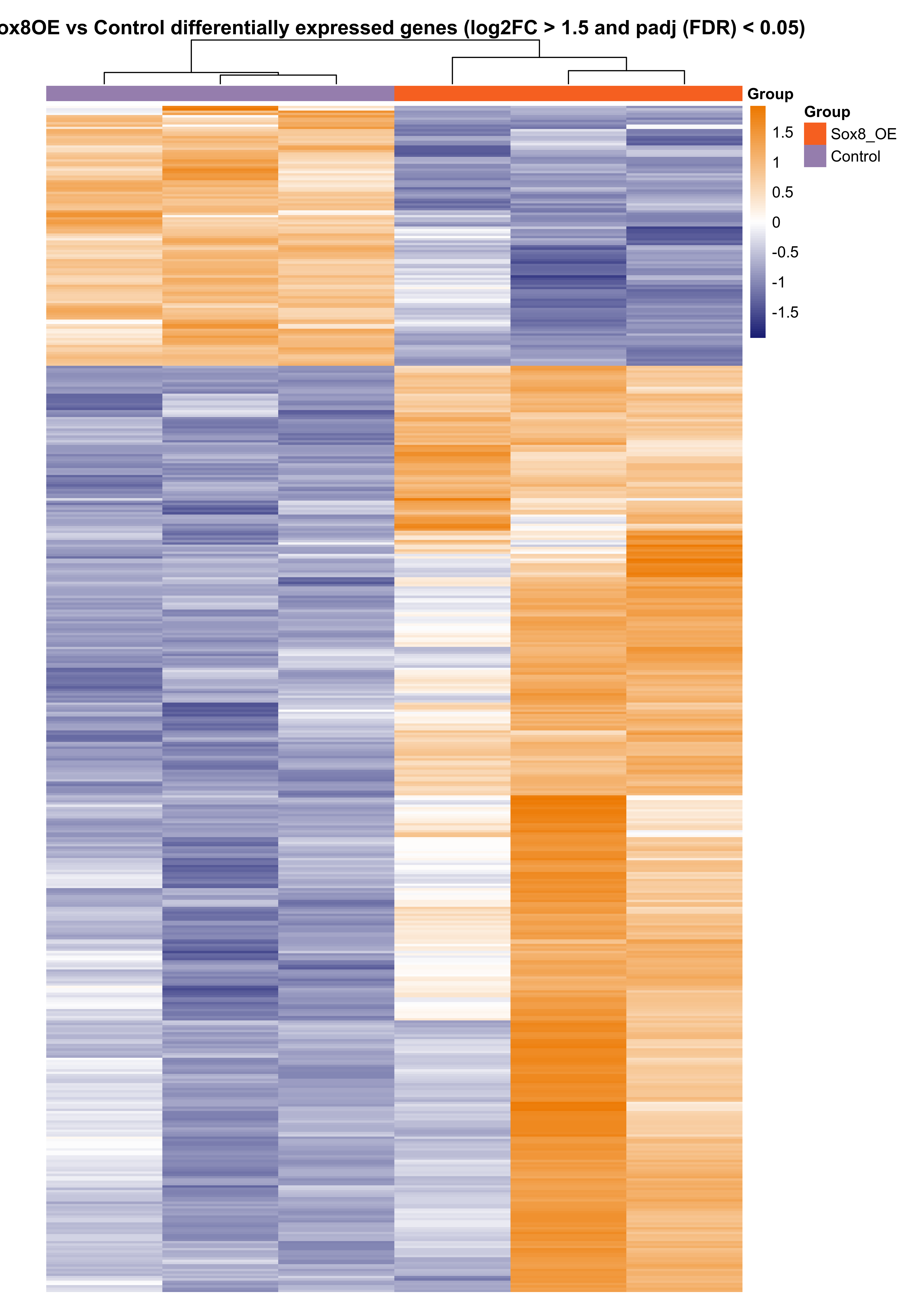
Subset differentially expressed genes (adjusted p-value < 0.05, absolute log2FC > 1.5).
res_sub <- res[which(res$padj < 0.05 & abs(res$log2FoldChange) > 1.5), ]
res_sub <- res_sub[order(-res_sub$log2FoldChange),]
Plot heatmap of differentially expressed genes.
png(paste0(output_path, "sox8_oe_hm.png"), height = 30, width = 21, family = 'Arial', units = "cm", res = 400)
pheatmap(assay(rld)[rownames(res_sub),], color = colorRampPalette(c("#191d73", "white", "#ed7901"))(n = 100), cluster_rows=T, show_rownames=FALSE,
         show_colnames = F, cluster_cols=T, annotation_col=as.data.frame(colData(deseq)["Group"]),
         annotation_colors = plot_colours, scale = "row", treeheight_row = 0, treeheight_col = 25,
         main = "Sox8OE vs Control differentially expressed genes (log2FC > 1.5 and padj (FDR) < 0.05)", border_color = NA, cellheight = 1.5, cellwidth = 75)
graphics.off()
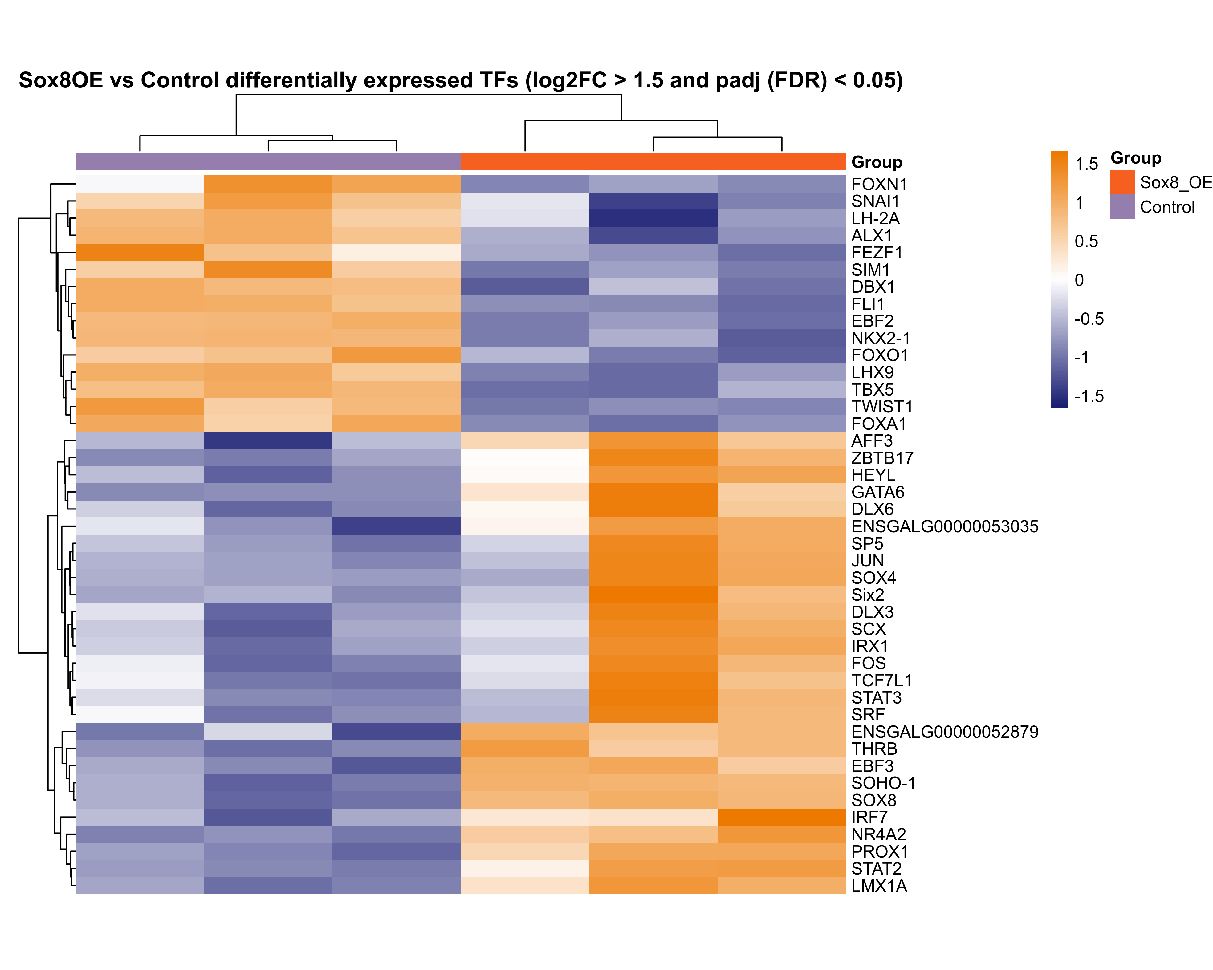
Subset differentially expressed transcription factors based on GO terms ('GO:0003700', 'GO:0043565', 'GO:0000981').
# Get biomart GO annotations for TFs
ensembl <- useEnsembl(biomart = 'ensembl',
                      dataset = 'ggallus_gene_ensembl',
                      version = 104)

TF_subset <- getBM(attributes=c("ensembl_gene_id", "go_id", "name_1006", "namespace_1003"),
                   filters = 'ensembl_gene_id',
                   values = rownames(res_sub),
                   mart = ensembl)

# subset genes based on transcription factor GO terms
TF_subset <- TF_subset$ensembl_gene_id[TF_subset$go_id %in% c('GO:0003700', 'GO:0043565', 'GO:0000981')]

res_sub_TF <- res_sub[rownames(res_sub) %in% TF_subset,]
Generate csv for raw counts, normalised counts, and differential expression output for transcription factors.
# subset TFs from all_dat
all_dat_TF <- all_dat[all_dat$gene_id %in% rownames(res_sub_TF),]

cat("This table shows differentially expressed (absolute FC > 1.5 and padj (FDR) < 0.05) transcription factors between Sox8 overexpression and control samples (Sox8 - Control)
Reads are aligned to Galgal6 \n
Statistics:
Normalised count: read counts adjusted for library size
pvalue: unadjusted pvalue for differential expression test between Sox8 overexpression and control samples
padj: pvalue for differential expression test between Sox8 overexpression and control samples - adjusted for multiple testing (Benjamini and Hochberg) \n \n",
    file = paste0(output_path, "Sox8_OE_SupplementaryData_6.csv"))
write.table(all_dat_TF, paste0(output_path, "Sox8_OE_SupplementaryData_6.csv"), append=TRUE, row.names = F, na = 'NA', sep=",")
Plot heatmap for differentially expressed transcription factors.
rld.plot <- assay(rld)
rownames(rld.plot) <- gene_annotations$gene_name[match(rownames(rld.plot), gene_annotations$gene_id)]

# plot DE TFs
png(paste0(output_path, "sox8_oe_TFs_hm.png"), height = 20, width = 25, family = 'Arial', units = "cm", res = 400)
pheatmap(rld.plot[res_sub_TF$gene_name,], color = colorRampPalette(c("#191d73", "white", "#ed7901"))(n = 100), cluster_rows=T, show_rownames=T,
                 show_colnames = F, cluster_cols=T, treeheight_row = 30, treeheight_col = 30,
                 annotation_col=as.data.frame(col_data["Group"]), annotation_colors = plot_colours,
                 scale = "row", main = "Sox8OE vs Control differentially expressed TFs (log2FC > 1.5 and padj (FDR) < 0.05)", border_color = NA,
                 cellheight = 10, cellwidth = 75)
graphics.off()
Compare DE data with DE TFs from Chen et al. (2017) Development
# Download supplementary file 4 from Chen et al. (2017)
# PPR vs otic 5/6ss, PPR vs otic 8/9ss, PPR vs otic 11/12ss. Dataset is already filtered for transcription factors

temp <- tempfile()
download.file("http://www.biologists.com/DEV_Movies/DEV148494/TableS4.xlsx", temp)

# read xlsx file
otic_enr <- read.xlsx(temp, startRow = 15)
unlink(temp)

# assign column names
colnames(otic_enr)[1:13] <- paste0(colnames(otic_enr)[1:13], c(rep('_normalised_count', 4), rep('_foldChange', 3),
                                                               rep('_pval', 3), rep('_padj', 3)))

# assign row names
rownames(otic_enr) <- otic_enr[,17]
otic_enr[,17] <- NULL

# remove genes from Chen dataset which are not DE in at least one of the stages (not sure why these are in the supplementary file)
otic_enr <- otic_enr[apply(otic_enr, 1, function(x) any(!is.na(x[c("5-6ss_foldChange", "8-9ss_foldChange", "11-12ss_foldChange")]))),]


# compare Sox8OE data vs otic enriched
# subset genes wich are 1.5FC between either PPR vs 4/5ss, PPR vs 8/9ss, PPR vs 11/12ss
otic_enr <- otic_enr[otic_enr$`5-6ss_foldChange` > 1.5 |
                       otic_enr$`8-9ss_foldChange` > 1.5 |
                       otic_enr$`11-12ss_foldChange` > 1.5,]
Plot venn diagram comparing OOPE and Sox8OE
venn.diagram(list(otic_enr=rownames(otic_enr), sox8OE=res_sub_TF$gene_name),
             category.names = c("logFC > 1.5 in any of PPR vs 5/6ss, PPR vs 8/9ss, PPR vs 11/12ss \n(Chen et al. 2017)", "Sox8OE enriched TFs\n(logFC > 1.5, padj = 0.05)"),
             filename = paste0(output_path, "otic_enriched_sox8OE_de_venn.png"),
             output = TRUE,
             imagetype = "png",
             height = 1100,
             width = 1100,
             resolution = 600,
             compression = "lzw",
             lwd = 1,
             col=c("#440154ff", '#21908dff'),
             fill = c(alpha("#440154ff",0.3), alpha('#21908dff',0.3)),
             cex = 0.5,
             fontfamily = "sans",
             cat.cex = 0.25,
             cat.pos = c(0, 0),
             cat.dist = c(0.03, 0.03),
             cat.fontfamily = "sans",
             cat.col = c("#440154ff", '#21908dff'),
             ext.percent = 0
)
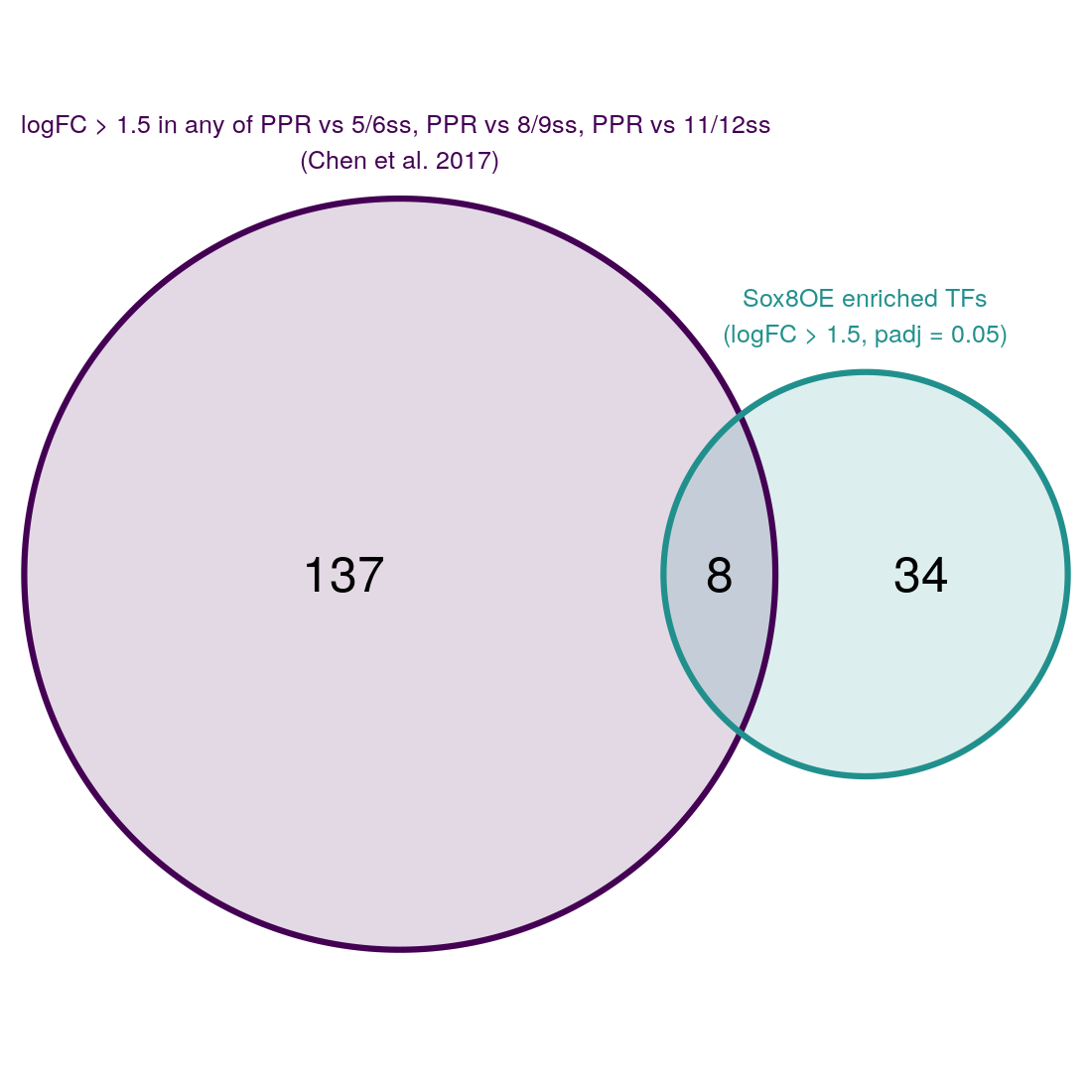
Make csv file of genes in each part of venn diagram
# when identifying shared genes between current study and previous studies which are alligned using different genome version, match genes using gene name.
# this is important as some of the Ensembl IDs from past genome versions have been depracated and therefore are absent from our data.
venn.genes <- list("Otic enriched" = rownames(otic_enr)[!rownames(otic_enr) %in% res_sub_TF$gene_name],
                   "Sox8OE" = res_sub_TF$gene_name[!res_sub_TF$gene_name %in% rownames(otic_enr)],
                   "Shared" = res_sub_TF$gene_name[res_sub_TF$gene_name %in% rownames(otic_enr)])

venn.genes.df <- t(plyr::ldply(venn.genes, rbind))
colnames(venn.genes.df) <- venn.genes.df[1,]
venn.genes.df <- venn.genes.df[-1,]


cat("This table provides a list of genes from each part of the venn diagram.
Differentially expressed transcription factors between Sox8 overexpression and control samples were cross compared with genes in supplementary table 4 of Chen et al. (2017) Development
Genes from supplementary table 4 of Chen et al. (2017) Development were filtered and kept if they were found to be differentially expressed (absolute FC > 1.5) between either: PPR vs 5/6ss otic; PPR vs 8/9ss otic; PPR vs 11/12ss otic \n \n",
    file = paste0(output_path, "Sox8_OE_process_output_2.csv"))
write.table(venn.genes.df, paste0(output_path, "Sox8_OE_process_output_2.csv"), append=TRUE, row.names = F, na = '', sep=",")
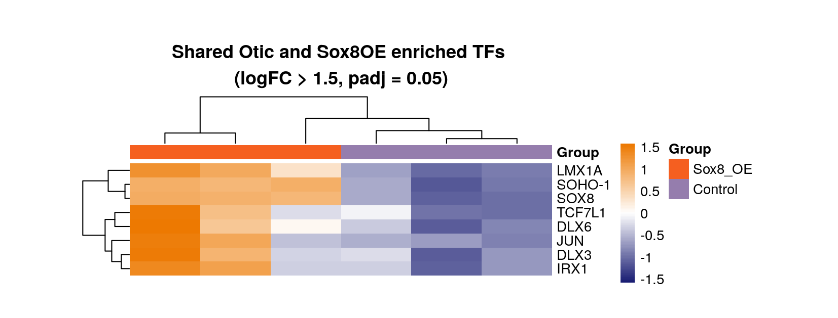
Plot heatmap of transcription factors which are DE in otic cells (Chen 2017) and DE in Sox8OE relative to control cells
rld.plot <- assay(rld)
rownames(rld.plot) <- gene_annotations$gene_name[match(rownames(rld.plot), gene_annotations$gene_id)]

png(paste0(output_path, "otic_enriched_sox8_de_hm.png"),height = 8, width = 21, units = "cm", res = 200)
pheatmap(rld.plot[venn.genes$Shared,], cluster_rows=T, show_rownames=T,
         show_colnames = F, cluster_cols=T, treeheight_row = 30, treeheight_col = 30,
         annotation_col=as.data.frame(col_data["Group"]), scale = "row",
         main = "Shared Otic and Sox8OE enriched TFs \n(logFC > 1.5, padj = 0.05)", cellwidth = 50, cellheight = 10,
         border_color = NA)
graphics.off()
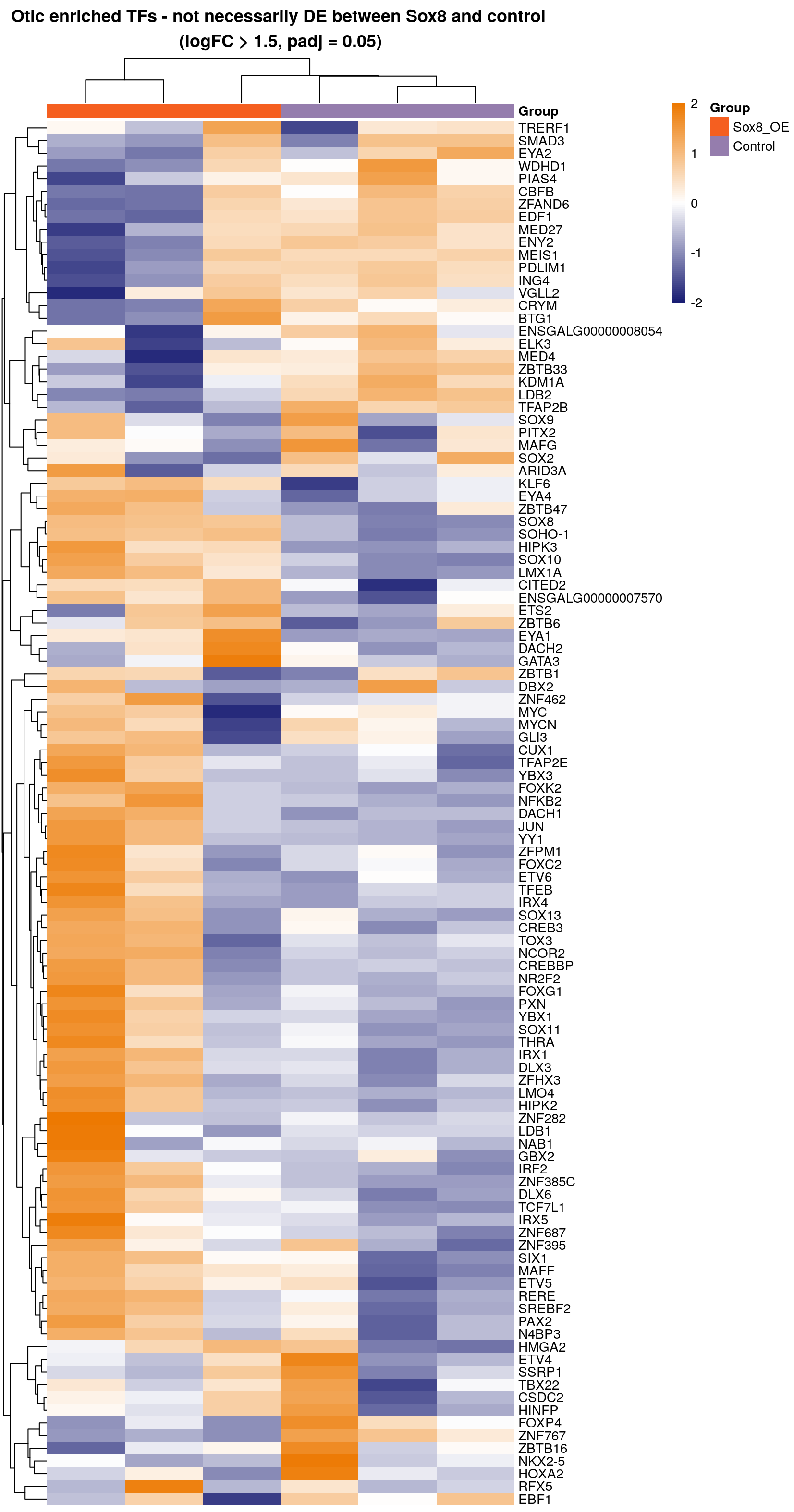
Plot all transcription factors DE in Chen et al. 2017 abs(1.5 FC) using our data - do not filter genes which are not DE in the Sox8OE
png(paste0(output_path, "otic_enriched_sox8_any_hm.png"),height = 40, width = 21, units = "cm", res = 200)
pheatmap(rld.plot[rownames(otic_enr)[rownames(otic_enr) %in% rownames(rld.plot)],], cluster_rows=T, show_rownames=T,
         show_colnames = F, cluster_cols=T, treeheight_row = 30, treeheight_col = 30,
         annotation_col=as.data.frame(col_data["Group"]), scale = "row",
         main = "Otic enriched TFs - not necessarily DE between Sox8 and control \n(logFC > 1.5, padj = 0.05)",
         border_color = NA)
graphics.off()

# This heatmap reveals that although many genes are not statistically DE in the Sox8OE - they are clearly upregulated in two of the three Sox8 samples.
# A possible explanation for this is that the Sox8OE does not necessarily switch on the otic program at the same rate in different samples and different cells.
# There may be modules of genes which are switched on at different points of otic specification. This variation could explain why these
# genes are not statistically differentially expressed.
Save CSV norm counts and Sox8OE DEA for genes from Chen et al. 2017
all_dat_Chen_DE <- all_dat[all_dat$gene_name %in% rownames(otic_enr),]


cat("This table shows genes subset from supplementary table 4 of Chen et al. (2017) Development
These genes were found to be differentially expressed (absolute FC > 1.5) between either: PPR vs 5/6ss otic; PPR vs 8/9ss otic; PPR vs 11/12ss otic
The data presented in this table are from Sox8 overexpression and control samples
Genes presented in this table are not necessarily differentially expressed between Sox8 overexpression and control samples \n
Statistics:
Normalised count: read counts adjusted for library size
pvalue: unadjusted pvalue for differential expression test between Sox8 overexpression and control samples
padj: pvalue for differential expression test between Sox8 overexpression and control samples - adjusted for multiple testing (Benjamini and Hochberg) \n \n",
    file = paste0(output_path, "Sox8_OE_process_output_3.csv"))
write.table(all_dat_Chen_DE, paste0(output_path, "Sox8_OE_process_output_3.csv"), append=TRUE, row.names = F, na = 'NA', sep=",")
norm counts and Sox8OE DEA for genes from Chen et al. 2017.
×